Hierarchicial Interferometric Bayesian Imaging (HIBI)

In this tutorial, we will demonstrate how to use Comrade to utilize Bayesian hierarchical modeling to reconstruct an image of M87. Regular imaging tries to make minimal assumptions about the source structure. We will demonstrate how a use can incorporate their knowledge of the source structure into the model to potentially improve the image reconstruction.

Explicitly, we will take advantage of the fact that optically thin accretion flows from a black hole that is face on is expected to produce a ring-like structure. To take advantage of this we will use a hierarchical imaging approach where we can easily incorporate this domain model into the image reconstruction.

This approach is called Hierarchical Interferometric Bayesian Imaging (HIBI) and is described in detail in the paper Hierarchical Interferometric Bayesian Imaging (in prep). For our image model we will use a raster image similar to Stokes I Simultaneous Image and Instrument Modeling. We will decompose the image raster components $F_{i j}$ as follows

F_{i j} = F_{0} \frac{μ (x_{i}, y_{j}) \exp (σ r_{i j})}{\sum_{i j} μ (x_{i}, y_{j}) \exp (σ r_{i j})}

where $F_{0}$ is the total flux of the image, $μ (x_{i}, y_{j})$ is a mean image and $r_{i j}$ is a is the multiplicative fluctuations about this mean image.

However, before we continue let's load the packages and tutorials we will need.

Loading the Data

To get started we will load Comrade

julia

using Comrade

Load the Data

julia

using VLBIFiles

For reproducibility we use a stable random number genreator

julia

using StableRNGs
rng = StableRNG(42)

StableRNGs.LehmerRNG(state=0x00000000000000000000000000000055)

To download the data visit https://doi.org/10.25739/g85n-f134

julia

uvd = VLBIFiles.load(
    VLBIFiles.UVData,
    joinpath(__DIR, "..", "..", "Data", "SR1_M87_2017_096_lo_hops_netcal_StokesI.uvfits")
)

VLBIFiles.UVData("/home/runner/work/Comrade.jl/Comrade.jl/examples/Data/SR1_M87_2017_096_lo_hops_netcal_StokesI.uvfits", VLBIFiles.UVHeader(SIMPLE  =                    T / conforms to FITS standard
BITPIX  =                  -32 / array data type
NAXIS   =                    7 / number of array dimensions
NAXIS1  =                    0
NAXIS2  =                    3
NAXIS3  =                    4
NAXIS4  =                    1
NAXIS5  =                    1
NAXIS6  =                    1
NAXIS7  =                    1
EXTEND  =                    T
GROUPS  =                    T / has groups
PCOUNT  =                    9 / number of parameters
GCOUNT  =                 8645 / number of groups
OBSRA   =    187.7059307575226
OBSDEC  =    12.39112323919932
OBJECT  = 'M87     '          
MJD     =              57849.0
DATE-OBS= '2017-04-06'        
BSCALE  =                  1.0
BZERO   =                  0.0
BUNIT   = 'JY      '          
VELREF  =                    3
EQUINOX = 'J2000   '          
ALTRPIX =                  1.0
ALTRVAL =                  0.0
TELESCOP= 'VLBA    '          
INSTRUME= 'VLBA    '          
OBSERVER= 'EHT     '          
CTYPE2  = 'COMPLEX '          
CRVAL2  =                  1.0
CDELT2  =                  1.0
CRPIX2  =                  1.0
CROTA2  =                  0.0
CTYPE3  = 'STOKES  '          
CRVAL3  =                 -1.0
CDELT3  =                 -1.0
CRPIX3  =                  1.0
CROTA3  =                  0.0
CTYPE4  = 'FREQ    '          
CRVAL4  =     2.27070703125e11
CDELT4  =              1.856e9
CRPIX4  =                  1.0
CROTA4  =                  0.0
CTYPE6  = 'RA      '          
CRVAL6  =    187.7059307575226
CDELT6  =                  1.0
CRPIX6  =                  1.0
CROTA6  =                  0.0
CTYPE7  = 'DEC     '          
CRVAL7  =    12.39112323919932
CDELT7  =                  1.0
CRPIX7  =                  1.0
CROTA7  =                  0.0
PTYPE1  = 'UU---SIN'          
PSCAL1  =  4.4039146672722e-12
PZERO1  =                  0.0
PTYPE2  = 'VV---SIN'          
PSCAL2  =  4.4039146672722e-12
PZERO2  =                  0.0
PTYPE3  = 'WW---SIN'          
PSCAL3  =  4.4039146672722e-12
PZERO3  =                  0.0
PTYPE4  = 'BASELINE'          
PSCAL4  =                  1.0
PZERO4  =                  0.0
PTYPE5  = 'DATE    '          
PSCAL5  =                  1.0
PZERO5  =                  0.0
PTYPE6  = 'DATE    '          
PSCAL6  =                  1.0
PZERO6  =                  0.0
PTYPE7  = 'INTTIM  '          
PSCAL7  =                  1.0
PZERO7  =                  0.0
PTYPE8  = 'TAU1    '          
PSCAL8  =                  1.0
PZERO8  =                  0.0
PTYPE9  = 'TAU2    '          
PSCAL9  =                  1.0
PZERO9  =                  0.0
HISTORY AIPS SORT ORDER='TB', "M87", Dates.Date("2017-04-06"), [:RR, :LL, :RL, :LR], 2.27070703125e11 Hz), VLBIFiles.FrequencyWindow[VLBIFiles.FrequencyWindow(1, 1, 2.270707f11 Hz, 1.856f9 Hz, 1, 1, 1.0f0)], VLBIFiles.AntArray[VLBIFiles.AntArray("VLBA", 2.270707f11 Hz, {1 = Antenna AA, 2 = Antenna AP, 3 = Antenna AZ, 4 = Antenna JC, 5 = Antenna LM, 6 = Antenna PV, 7 = Antenna SM, 8 = Antenna SR}, [0.0, 0.0, 0.0])])

For this tutorial we will once again fit complex visibilities since they provide the most information once the telescope/instrument model are taken into account. We scan-average the data (gain phases are coherent within a scan), then remove baselines shorter than 0.1Gλ and add 1% systematic uncertainty to handle residual calibration errors such as leakage.

julia

dvis = extract_table(uvd, Visibilities(; time_average = VLBI.GapBasedScans()))
dvis = flag(x -> uvdist(x) < 0.1e9, dvis)
add_fractional_noise!(dvis, 0.01)

EHTObservationTable{Comrade.EHTVisibilityDatum{:I}}
  source:      M87
  mjd:         57849
  bandwidth:   1.856e9
  sites:       [:AA, :AP, :AZ, :JC, :LM, :PV, :SM]
  nsamples:    242

Building the Model/Posterior

Now let's construct our model using the decomposition described above. We use the @sky macro to define the model and prior in a single block. Each name ~ dist line contributes an entry to the prior; everything else is the model body. The uniform priors on r, ain, aout are the ring radius and inner/outer radial brightness power-law indices. σimg is half-normal to keep the MRF close to the mean image.

julia

using VLBIImagePriors
using Distributions
@sky function sky(grid; ftot, cprior)
    c ~ cprior
    σimg ~ VLBITruncated(VLBIGaussian(0.0, 0.5); lower = 0.0)
    r ~ VLBIUniform(μas2rad(10.0), μas2rad(40.0))
    ain ~ VLBIUniform(1.0, 20.0)
    aout ~ VLBIUniform(1.0, 20.0)
    # Form the image model
    mb = RingTemplate(RadialDblPower(ain, aout), AzimuthalUniform())
    mr = modify(mb, Stretch(r))
    mimg = intensitymap(mr, grid)
    rast = apply_fluctuations(CenteredLR(), mimg, σimg * c.params)
    rast .*= ftot
    mimg = ContinuousImage(rast, grid, BSplinePulse{3}())
    return mimg
end

sky (generic function with 1 method)

Unlike other imaging examples (e.g., Imaging a Black Hole using only Closure Quantities) we also need to include a model for the instrument, i.e., gains as well. The gains will be broken into two components

Gain amplitudes which are typically known to 10-20%, except for LMT, which has amplitudes closer to 50-100%.
Gain phases which are more difficult to constrain and can shift rapidly.

julia

using VLBIImagePriors
using Distributions
fgain(x) = exp(complex(x.lg, x.gp))
G = SingleStokesGain(fgain)

intpr = (
    lg = ArrayPrior(IIDSitePrior(ScanSeg(), VLBIGaussian(0.0, 0.2)); LM = IIDSitePrior(ScanSeg(), VLBIGaussian(0.0, 1.0))),
    gp = ArrayPrior(IIDSitePrior(ScanSeg(), DiagonalVonMises(0.0, inv(π^2))); refant = SEFDReference(0.0)),
)
intmodel = InstrumentModel(G, intpr)

InstrumentModel
  with Jones: SingleStokesGain
  with reference basis: PolarizedTypes.CirBasis()

Now let's define our grid and the data-dependent prior, then build the sky model.

julia

fovxy = μas2rad(150.0)
npix = 48
g = imagepixels(fovxy, fovxy, npix, npix)

RectiGrid(
executor: ComradeBase.Serial()
Dimensions: 
(↓ X Sampled{Float64} LinRange{Float64}(-3.560350470648155e-10, 3.560350470648155e-10, 48) ForwardOrdered Regular Points,
→ Y Sampled{Float64} LinRange{Float64}(-3.560350470648155e-10, 3.560350470648155e-10, 48) ForwardOrdered Regular Points)
)

Part of hybrid imaging is to force a scale separation between the different model components to make them identifiable. To enforce this we will set the raster component to have a correlation length of 5 times the beam size.

julia

cprior = corr_image_prior(g, dvis)

skym = sky(g; ftot = 1.1, cprior)

SkyModel
  with map: _sky_sky
   on grid: 
RectiGrid(
executor: ComradeBase.Serial()
Dimensions: 
(↓ X Sampled{Float64} LinRange{Float64}(-3.560350470648155e-10, 3.560350470648155e-10, 48) ForwardOrdered Regular Points,
→ Y Sampled{Float64} LinRange{Float64}(-3.560350470648155e-10, 3.560350470648155e-10, 48) ForwardOrdered Regular Points)
)
   )

This is everything we need to specify our posterior distribution, which our is the main object of interest in image reconstructions when using Bayesian inference.

julia

using Enzyme
post = VLBIPosterior(skym, intmodel, dvis);

We can sample from the prior to see what the model looks like

julia

using CairoMakie
xrand = prior_sample(rng, post)
gpl = refinespatial(g, 3)
fig = imageviz(intensitymap(skymodel(post, xrand), gpl));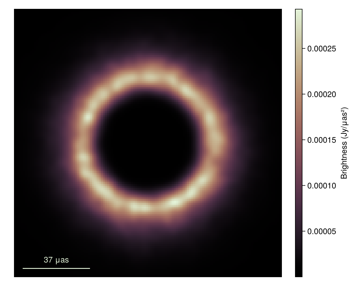

Reconstructing the Image

To find the image we will demonstrate two methods:

Optimization to find the MAP (fast but often a poor estimator)
Sampling to find the posterior (slow but provides a substantially better estimator)

For optimization we will use the Optimization.jl package and the LBFGS optimizer. To use this we use the comrade_opt function

julia

using Optimization, OptimizationLBFGSB
xopt, sol = comrade_opt(
    post, LBFGSB();
    initial_params = xrand, maxiters = 2000, g_tol = 1.0e0
);

First we will evaluate our fit by plotting the residuals

julia

res = residuals(post, xopt);
fig = plotfields(res[1], :uvdist, :res);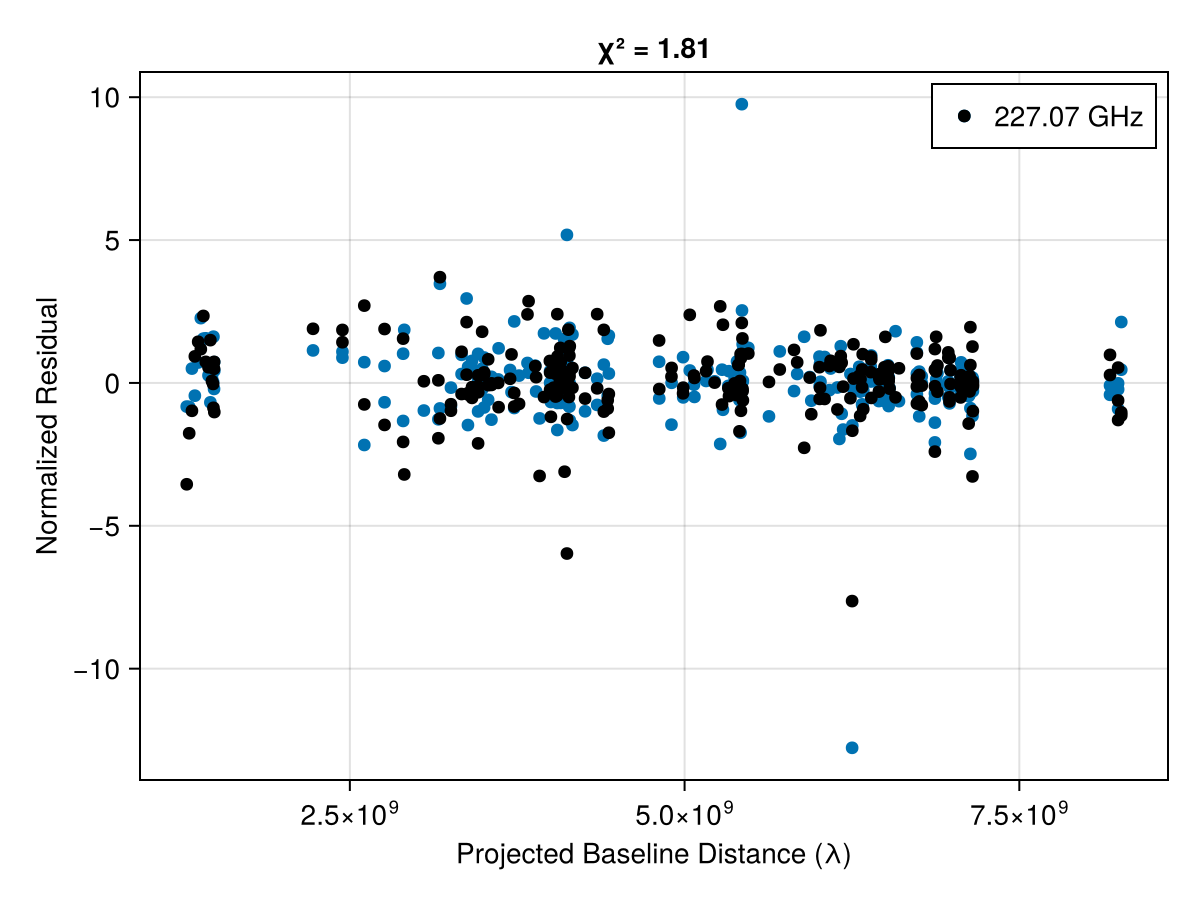

These residuals suggest that we are substantially overfitting the data. This is a common side effect of MAP imaging. As a result if we plot the image we see that there is substantial high-frequency structure in the image that isn't supported by the data.

julia

fig = imageviz(intensitymap(skymodel(post, xopt), gpl), figure = (; resolution = (500, 400)));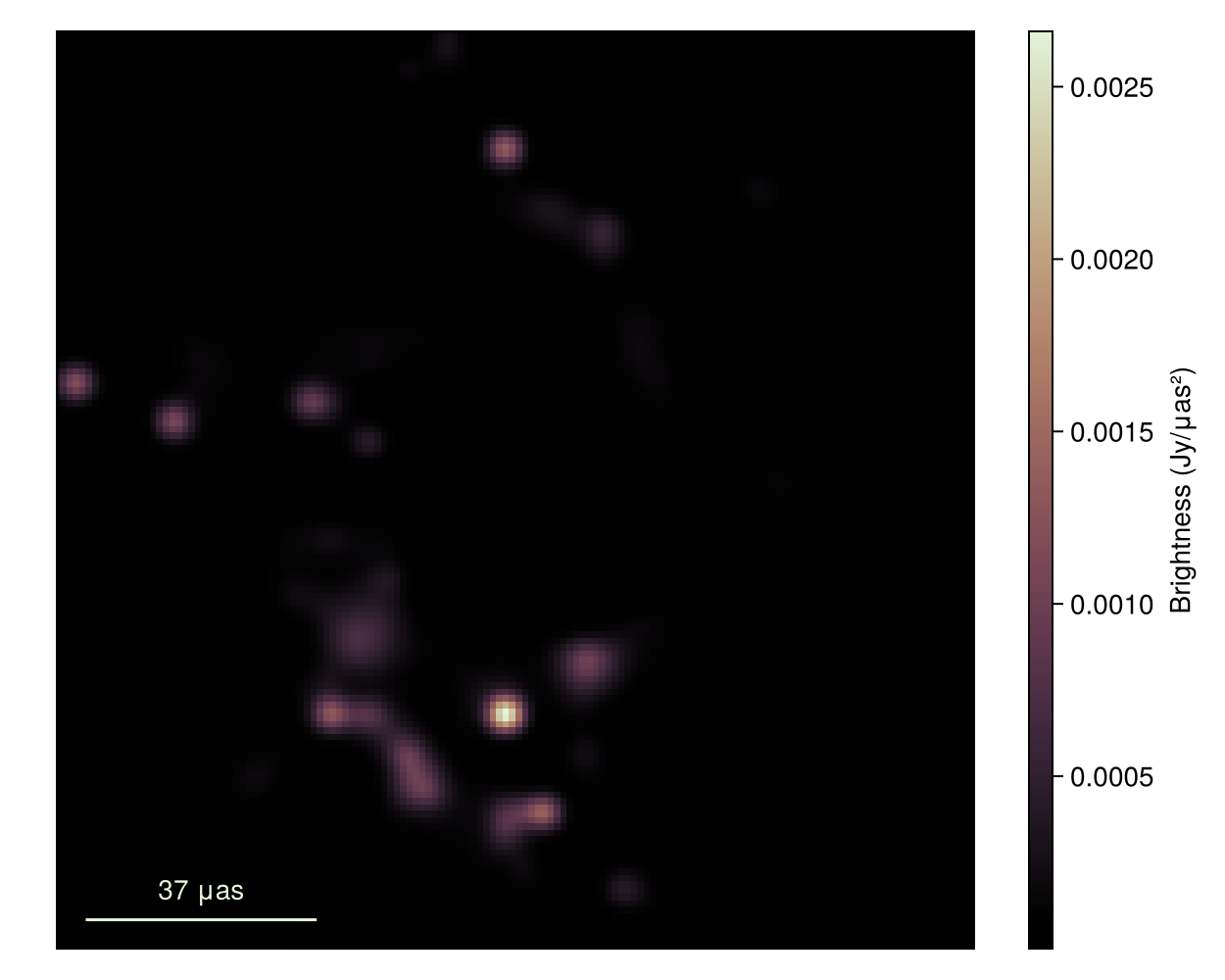

To improve our results we will now move to Posterior sampling. This is the main method we recommend for all inference problems in Comrade. While it is slower the results are often substantially better. To sample we will use the AdvancedHMC package.

julia

using AdvancedHMC
chain = sample(rng, post, NUTS(0.8), 700; n_adapts = 500, progress = false, initial_params = xopt);

[ Info: Found initial step size 0.000390625

chain = load_samples(out) We then remove the adaptation/warmup phase from our chain

julia

chain = chain[501:end]

PosteriorSamples
  Samples size: (200,)
  sampler used: AHMC
                                      Mean
┌───────────────────────────────────────────────────────────────────────────────
│ sky                                                                          ⋯
│ @NamedTuple{c::@NamedTuple{params::Matrix{Float64}, hyperparams::Float64}, σ ⋯
├───────────────────────────────────────────────────────────────────────────────
│ (c = (params = [0.14423 0.174735 … -0.138515 -0.025456; 0.122132 0.098365 …  ⋯
└───────────────────────────────────────────────────────────────────────────────
                                                               2 columns omitted
                                   Std. Dev.
┌───────────────────────────────────────────────────────────────────────────────
│ sky                                                                          ⋯
│ @NamedTuple{c::@NamedTuple{params::Matrix{Float64}, hyperparams::Float64}, σ ⋯
├───────────────────────────────────────────────────────────────────────────────
│ (c = (params = [0.63957 0.665592 … 0.574833 0.555357; 0.593687 0.694525 … 0. ⋯
└───────────────────────────────────────────────────────────────────────────────
                                                               2 columns omitted

Warning

This should be run for 4-5x more steps to properly estimate expectations of the posterior

Now lets plot the mean image and standard deviation images. To do this we first clip the first 250 MCMC steps since that is during tuning and so the posterior is not sampling from the correct sitesary distribution.

julia

using StatsBase
msamples = skymodel.(Ref(post), chain[begin:5:end]);

WARNING: using StatsBase.residuals in module ##225 conflicts with an existing identifier.

The mean image is then given by

julia

imgs = intensitymap.(msamples, Ref(gpl))
fig = imageviz(mean(imgs), size = (400, 300));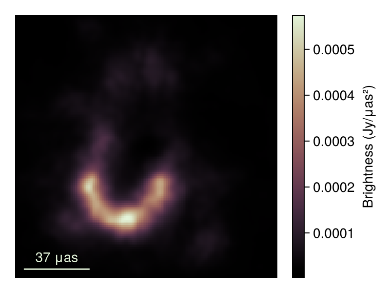

julia

fig = imageviz(std(imgs), colormap = :batlow, size = (400, 300));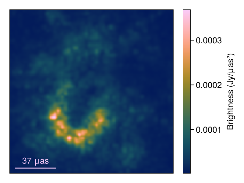

Finally, let's take a look at some of the ring parameters

julia

figd = Figure(; resolution = (650, 200));
p1 = density(figd[1, 1], rad2μas(chain.sky.r) * 2, axis = (xlabel = "Ring Pwr Law Transition (μas)",))
p2 = density(figd[1, 2], chain.sky.ain, axis = (xlabel = "Inner Radial Index",))
p3 = density(figd[1, 3], chain.sky.aout, axis = (xlabel = "Outer Radial Index",))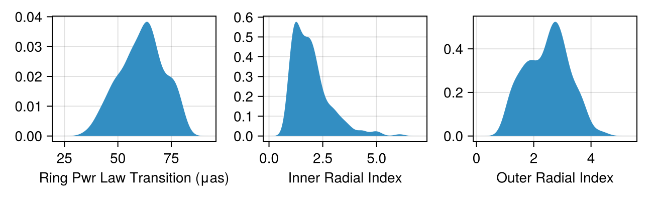

Now let's check the residuals using draws from the posterior

julia

fig = Figure(; size = (600, 400))
resch = residuals(post, chain[end])
ax, = plotfields!(fig[1, 1], resch[1], :uvdist, :res, scatter_kwargs = (; label = "MAP", color = :blue, colorim = :red, marker = :circle), legend = false)
for s in sample(chain, 10)
    baselineplot!(ax, residuals(post, s)[1], :uvdist, :res, alpha = 0.2, label = "Draw")
end
axislegend(ax, merge = true)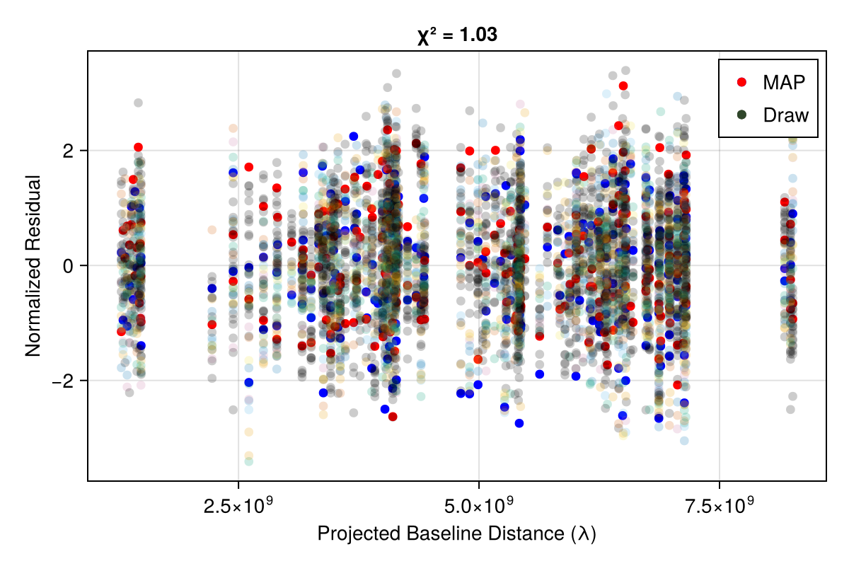

This page was generated using Literate.jl.

Hierarchicial Interferometric Bayesian Imaging (HIBI) ​

Loading the Data ​

Load the Data ​

Building the Model/Posterior ​

Reconstructing the Image ​

Hierarchicial Interferometric Bayesian Imaging (HIBI)

Loading the Data

Load the Data

Building the Model/Posterior

Reconstructing the Image