Stokes I Simultaneous Image and Instrument Modeling
In this tutorial, we will create a preliminary reconstruction of the 2017 M87 data on April 6 by simultaneously creating an image and model for the instrument. By instrument model, we mean something akin to self-calibration in traditional VLBI imaging terminology. However, unlike traditional self-cal, we will solve for the gains each time we update the image self-consistently. This allows us to model the correlations between gains and the image.
To get started we load Comrade.
using Comrade


using VLBIFiles
using LinearAlgebra
For reproducibility we use a stable random number genreator
using StableRNGs
rng = StableRNG(42)StableRNGs.LehmerRNG(state=0x00000000000000000000000000000055)Load the Data
To download the data visit https://doi.org/10.25739/g85n-f134 First we will load our data:
uvd = VLBIFiles.load(
    VLBIFiles.UVData,
    joinpath(__DIR, "..", "..", "Data", "SR1_M87_2017_096_lo_hops_netcal_StokesI.uvfits")
)
VLBIFiles.UVData("/home/runner/work/Comrade.jl/Comrade.jl/examples/Data/SR1_M87_2017_096_lo_hops_netcal_StokesI.uvfits", VLBIFiles.UVHeader(SIMPLE = T / conforms to FITS standard
BITPIX = -32 / array data type
NAXIS = 7 / number of array dimensions
NAXIS1 = 0
NAXIS2 = 3
NAXIS3 = 4
NAXIS4 = 1
NAXIS5 = 1
NAXIS6 = 1
NAXIS7 = 1
EXTEND = T
GROUPS = T / has groups
PCOUNT = 9 / number of parameters
GCOUNT = 8645 / number of groups
OBSRA = 187.7059307575226
OBSDEC = 12.39112323919932
OBJECT = 'M87 '
MJD = 57849.0
DATE-OBS= '2017-04-06'
BSCALE = 1.0
BZERO = 0.0
BUNIT = 'JY '
VELREF = 3
EQUINOX = 'J2000 '
ALTRPIX = 1.0
ALTRVAL = 0.0
TELESCOP= 'VLBA '
INSTRUME= 'VLBA '
OBSERVER= 'EHT '
CTYPE2 = 'COMPLEX '
CRVAL2 = 1.0
CDELT2 = 1.0
CRPIX2 = 1.0
CROTA2 = 0.0
CTYPE3 = 'STOKES '
CRVAL3 = -1.0
CDELT3 = -1.0
CRPIX3 = 1.0
CROTA3 = 0.0
CTYPE4 = 'FREQ '
CRVAL4 = 2.27070703125e11
CDELT4 = 1.856e9
CRPIX4 = 1.0
CROTA4 = 0.0
CTYPE6 = 'RA '
CRVAL6 = 187.7059307575226
CDELT6 = 1.0
CRPIX6 = 1.0
CROTA6 = 0.0
CTYPE7 = 'DEC '
CRVAL7 = 12.39112323919932
CDELT7 = 1.0
CRPIX7 = 1.0
CROTA7 = 0.0
PTYPE1 = 'UU---SIN'
PSCAL1 = 4.4039146672722e-12
PZERO1 = 0.0
PTYPE2 = 'VV---SIN'
PSCAL2 = 4.4039146672722e-12
PZERO2 = 0.0
PTYPE3 = 'WW---SIN'
PSCAL3 = 4.4039146672722e-12
PZERO3 = 0.0
PTYPE4 = 'BASELINE'
PSCAL4 = 1.0
PZERO4 = 0.0
PTYPE5 = 'DATE '
PSCAL5 = 1.0
PZERO5 = 0.0
PTYPE6 = 'DATE '
PSCAL6 = 1.0
PZERO6 = 0.0
PTYPE7 = 'INTTIM '
PSCAL7 = 1.0
PZERO7 = 0.0
PTYPE8 = 'TAU1 '
PSCAL8 = 1.0
PZERO8 = 0.0
PTYPE9 = 'TAU2 '
PSCAL9 = 1.0
PZERO9 = 0.0
HISTORY AIPS SORT ORDER='TB', "M87", Dates.Date("2017-04-06"), [:RR, :LL, :RL, :LR], 2.27070703125e11 Hz), VLBIFiles.FrequencyWindow[VLBIFiles.FrequencyWindow(1, 1, 2.270707f11 Hz, 1.856f9 Hz, 1, 1, 1.0f0)], VLBIFiles.AntArray[VLBIFiles.AntArray("VLBA", 2.270707f11 Hz, {1 = Antenna AA, 2 = Antenna AP, 3 = Antenna AZ, 4 = Antenna JC, 5 = Antenna LM, 6 = Antenna PV, 7 = Antenna SM, 8 = Antenna SR}, [0.0, 0.0, 0.0])])Extract scan-averaged complex visibilities. Then inflate the noise by 2% to account for residual calibration errors.
dvis = extract_table(uvd, Visibilities(; time_average = VLBI.GapBasedScans()))
add_fractional_noise!(dvis, 0.02)
EHTObservationTable{Comrade.EHTVisibilityDatum{:I}}
source: M87
mjd: 57849
bandwidth: 1.856e9
sites: [:AA, :AP, :AZ, :JC, :LM, :PV, :SM]
nsamples: 274##Building the Model/Posterior
Now, we must build our intensity/visibility model. That is, the model that takes in a named tuple of parameters and perhaps some metadata required to construct the model. For our model, we will use a raster or ContinuousImage for our image model. The model is given below:
The model construction is very similar to Imaging a Black Hole using only Closure Quantities, except we include a large scale gaussian since we want to model the zero baselines. For more information about the image model please read the closure-only example. We use the @sky macro to bundle the model and its priors in one block. Each name ~ dist line adds an entry to the prior; everything else is the model body.
using VLBIImagePriors
using Distributions
@sky function sky(grid; ftot, mimg, cprior)
    c ~ cprior
    σimg ~ VLBITruncated(VLBIGaussian(0.0, 0.5); lower = 0.0)
    fg ~ VLBIUniform(0.0, 1.0)
    # Apply the GMRF fluctuations to the image
    rast = apply_fluctuations(CenteredLR(), mimg, σimg .* c.params)
    pimg = parent(rast)
    @. pimg = (ftot * (1 - fg)) * pimg
    m = ContinuousImage(rast, BSplinePulse{3}())
    # Add a large-scale gaussian to deal with the over-resolved mas flux
    g = modify(Gaussian(), Stretch(μas2rad(500.0), μas2rad(500.0)), Renormalize(ftot * fg))
    x, y = centroid(m)
    return shifted(m, -x, -y) + g
end
sky (generic function with 1 method)Now, let's set up our image model. The EHT's nominal resolution is 20-25 μas. Additionally, the EHT is not very sensitive to a larger field of view. Typically 60-80 μas is enough to describe the compact flux of M87. Given this, we only need to use a small number of pixels to describe our image.
npix = 48
fovx = μas2rad(200.0)
fovy = μas2rad(200.0)9.69627362219072e-10Now let's form our cache's. First, we have our usual image cache which is needed to numerically compute the visibilities.
grid = imagepixels(fovx, fovy, npix, npix)RectiGrid(
executor: ComradeBase.Serial()
Dimensions:
(↓ X Sampled{Float64} LinRange{Float64}(-4.747133960864206e-10, 4.747133960864206e-10, 48) ForwardOrdered Regular Points,
→ Y Sampled{Float64} LinRange{Float64}(-4.747133960864206e-10, 4.747133960864206e-10, 48) ForwardOrdered Regular Points)
)Since we are using a Gaussian Markov random field prior we need to first specify our mean image. This behaves somewhat similary to a entropy regularizer in that it will start with an initial guess for the image structure. For this tutorial we will use a a symmetric Gaussian with a FWHM of 50 μas
fwhmfac = 2 * sqrt(2 * log(2))
mpr = modify(Gaussian(), Stretch(μas2rad(60.0) ./ fwhmfac))
mimg_raw = intensitymap(mpr, grid)
mimg = mimg_raw ./ Comrade.flux(mimg_raw)┌ 48×48 IntensityMap{Float64, 2} ┐
├────────────────────────────────┴─────────────────────────────────────── dims ┐
↓ X Sampled{Float64} LinRange{Float64}(-4.747133960864206e-10, 4.747133960864206e-10, 48) ForwardOrdered Regular Points,
→ Y Sampled{Float64} LinRange{Float64}(-4.747133960864206e-10, 4.747133960864206e-10, 48) ForwardOrdered Regular Points
└──────────────────────────────────────────────────────────────────────────────┘
↓ → -4.74713e-10 -4.54513e-10 -4.34312e-10 -4.14112e-10 -3.93911e-10 -3.73711e-10 -3.5351e-10 -3.33309e-10 -3.13109e-10 -2.92908e-10 -2.72708e-10 -2.52507e-10 -2.32307e-10 -2.12106e-10 -1.91905e-10 -1.71705e-10 -1.51504e-10 -1.31304e-10 -1.11103e-10 -9.09026e-11 -7.0702e-11 -5.05014e-11 -3.03009e-11 -1.01003e-11 1.01003e-11 3.03009e-11 5.05014e-11 7.0702e-11 9.09026e-11 1.11103e-10 1.31304e-10 1.51504e-10 1.71705e-10 1.91905e-10 2.12106e-10 2.32307e-10 2.52507e-10 2.72708e-10 2.92908e-10 3.13109e-10 3.33309e-10 3.5351e-10 3.73711e-10 3.93911e-10 4.14112e-10 4.34312e-10 4.54513e-10 4.74713e-10
-4.74713e-10 1.64194e-9 3.03721e-9 5.46989e-9 9.59111e-9 1.63736e-8 2.72149e-8 4.40409e-8 6.9389e-8 1.06442e-7 1.58971e-7 2.3116e-7 3.27259e-7 4.51084e-7 6.05354e-7 7.90948e-7 1.00617e-6 1.24618e-6 1.50272e-6 1.76426e-6 2.01665e-6 2.24433e-6 2.4318e-6 2.5654e-6 2.63493e-6 2.63493e-6 2.5654e-6 2.4318e-6 2.24433e-6 2.01665e-6 1.76426e-6 1.50272e-6 1.24618e-6 1.00617e-6 7.90948e-7 6.05354e-7 4.51084e-7 3.27259e-7 2.3116e-7 1.58971e-7 1.06442e-7 6.9389e-8 4.40409e-8 2.72149e-8 1.63736e-8 9.59111e-9 5.46989e-9 3.03721e-9 1.64194e-9
-4.54513e-10 3.03721e-9 5.61814e-9 1.0118e-8 1.77413e-8 3.02874e-8 5.03414e-8 8.14655e-8 1.28354e-7 1.96893e-7 2.9406e-7 4.27592e-7 6.05354e-7 8.34402e-7 1.11977e-6 1.46307e-6 1.86119e-6 2.30516e-6 2.77969e-6 3.26347e-6 3.73034e-6 4.15149e-6 4.49827e-6 4.7454e-6 4.87402e-6 4.87402e-6 4.7454e-6 4.49827e-6 4.15149e-6 3.73034e-6 3.26347e-6 2.77969e-6 2.30516e-6 1.86119e-6 1.46307e-6 1.11977e-6 8.34402e-7 6.05354e-7 4.27592e-7 2.9406e-7 1.96893e-7 1.28354e-7 8.14655e-8 5.03414e-8 3.02874e-8 1.77413e-8 1.0118e-8 5.61814e-9 3.03721e-9
-4.34312e-10 5.46989e-9 1.0118e-8 1.82222e-8 3.19514e-8 5.45465e-8 9.06628e-8 1.46716e-7 2.3116e-7 3.54596e-7 5.29591e-7 7.70077e-7 1.09022e-6 1.50272e-6 2.01665e-6 2.63493e-6 3.35192e-6 4.15149e-6 5.00611e-6 5.87738e-6 6.7182e-6 7.47666e-6 8.1012e-6 8.54628e-6 8.7779e-6 8.7779e-6 8.54628e-6 8.1012e-6 7.47666e-6 6.7182e-6 5.87738e-6 5.00611e-6 4.15149e-6 3.35192e-6 2.63493e-6 2.01665e-6 1.50272e-6 1.09022e-6 7.70077e-7 5.29591e-7 3.54596e-7 2.3116e-7 1.46716e-7 9.06628e-8 5.45465e-8 3.19514e-8 1.82222e-8 1.0118e-8 5.46989e-9
-4.14112e-10 9.59111e-9 1.77413e-8 3.19514e-8 5.60248e-8 9.56437e-8 1.58971e-7 2.57257e-7 4.05324e-7 6.21761e-7 9.28604e-7 1.35028e-6 1.91163e-6 2.63493e-6 3.53607e-6 4.62018e-6 5.87738e-6 7.27937e-6 8.7779e-6 1.03056e-5 1.17799e-5 1.31099e-5 1.42049e-5 1.49854e-5 1.53915e-5 1.53915e-5 1.49854e-5 1.42049e-5 1.31099e-5 1.17799e-5 1.03056e-5 8.7779e-6 7.27937e-6 5.87738e-6 4.62018e-6 3.53607e-6 2.63493e-6 1.91163e-6 1.35028e-6 9.28604e-7 6.21761e-7 4.05324e-7 2.57257e-7 1.58971e-7 9.56437e-8 5.60248e-8 3.19514e-8 1.77413e-8 9.59111e-9
-3.93911e-10 1.63736e-8 3.02874e-8 5.45465e-8 9.56437e-8 1.6328e-7 2.71391e-7 4.39181e-7 6.91956e-7 1.06145e-6 1.58528e-6 2.30516e-6 3.26347e-6 4.49827e-6 6.03667e-6 7.88743e-6 1.00337e-5 1.24271e-5 1.49854e-5 1.75934e-5 2.01103e-5 2.23807e-5 2.42502e-5 2.55825e-5 2.62759e-5 2.62759e-5 2.55825e-5 2.42502e-5 2.23807e-5 2.01103e-5 1.75934e-5 1.49854e-5 1.24271e-5 1.00337e-5 7.88743e-6 6.03667e-6 4.49827e-6 3.26347e-6 2.30516e-6 1.58528e-6 1.06145e-6 6.91956e-7 4.39181e-7 2.71391e-7 1.6328e-7 9.56437e-8 5.45465e-8 3.02874e-8 1.63736e-8
-3.73711e-10 2.72149e-8 5.03414e-8 9.06628e-8 1.58971e-7 2.71391e-7 4.51084e-7 7.29972e-7 1.15011e-6 1.76426e-6 2.63493e-6 3.83144e-6 5.42428e-6 7.47666e-6 1.00337e-5 1.31099e-5 1.66772e-5 2.06554e-5 2.49075e-5 2.92423e-5 3.34258e-5 3.71995e-5 4.03068e-5 4.25212e-5 4.36736e-5 4.36736e-5 4.25212e-5 4.03068e-5 3.71995e-5 3.34258e-5 2.92423e-5 2.49075e-5 2.06554e-5 1.66772e-5 1.31099e-5 1.00337e-5 7.47666e-6 5.42428e-6 3.83144e-6 2.63493e-6 1.76426e-6 1.15011e-6 7.29972e-7 4.51084e-7 2.71391e-7 1.58971e-7 9.06628e-8 5.03414e-8 2.72149e-8
-3.5351e-10 4.40409e-8 8.14655e-8 1.46716e-7 2.57257e-7 4.39181e-7 7.29972e-7 1.18129e-6 1.86119e-6 2.85503e-6 4.26401e-6 6.20028e-6 8.7779e-6 1.20992e-5 1.62371e-5 2.12152e-5 2.6988e-5 3.34258e-5 4.03068e-5 4.73218e-5 5.40916e-5 6.01984e-5 6.52269e-5 6.88104e-5 7.06754e-5 7.06754e-5 6.88104e-5 6.52269e-5 6.01984e-5 5.40916e-5 4.73218e-5 4.03068e-5 3.34258e-5 2.6988e-5 2.12152e-5 1.62371e-5 1.20992e-5 8.7779e-6 6.20028e-6 4.26401e-6 2.85503e-6 1.86119e-6 1.18129e-6 7.29972e-7 4.39181e-7 2.57257e-7 1.46716e-7 8.14655e-8 4.40409e-8
-3.33309e-10 6.9389e-8 1.28354e-7 2.3116e-7 4.05324e-7 6.91956e-7 1.15011e-6 1.86119e-6 2.93241e-6 4.49827e-6 6.7182e-6 9.76891e-6 1.38301e-5 1.9063e-5 2.55825e-5 3.34258e-5 4.25212e-5 5.26643e-5 6.35057e-5 7.45582e-5 8.52246e-5 9.48462e-5 0.000102769 0.000108415 0.000111353 0.000111353 0.000108415 0.000102769 9.48462e-5 8.52246e-5 7.45582e-5 6.35057e-5 5.26643e-5 4.25212e-5 3.34258e-5 2.55825e-5 1.9063e-5 1.38301e-5 9.76891e-6 6.7182e-6 4.49827e-6 2.93241e-6 1.86119e-6 1.15011e-6 6.91956e-7 4.05324e-7 2.3116e-7 1.28354e-7 6.9389e-8
-3.13109e-10 1.06442e-7 1.96893e-7 3.54596e-7 6.21761e-7 1.06145e-6 1.76426e-6 2.85503e-6 4.49827e-6 6.90028e-6 1.03056e-5 1.49854e-5 2.12152e-5 2.92423e-5 3.92432e-5 5.12746e-5 6.52269e-5 8.07862e-5 9.74168e-5 0.000114371 0.000130733 0.000145493 0.000157646 0.000166307 0.000170814 0.000170814 0.000166307 0.000157646 0.000145493 0.000130733 0.000114371 9.74168e-5 8.07862e-5 6.52269e-5 5.12746e-5 3.92432e-5 2.92423e-5 2.12152e-5 1.49854e-5 1.03056e-5 6.90028e-6 4.49827e-6 2.85503e-6 1.76426e-6 1.06145e-6 6.21761e-7 3.54596e-7 1.96893e-7 1.06442e-7
-2.92908e-10 1.58971e-7 2.9406e-7 5.29591e-7 9.28604e-7 1.58528e-6 2.63493e-6 4.26401e-6 6.7182e-6 1.03056e-5 1.53915e-5 2.23807e-5 3.1685e-5 4.36736e-5 5.861e-5 7.6579e-5 9.74168e-5 0.000120655 0.000145493 0.000170814 0.000195251 0.000217294 0.000235445 0.00024838 0.000255112 0.000255112 0.00024838 0.000235445 0.000217294 0.000195251 0.000170814 0.000145493 0.000120655 9.74168e-5 7.6579e-5 5.861e-5 4.36736e-5 3.1685e-5 2.23807e-5 1.53915e-5 1.03056e-5 6.7182e-6 4.26401e-6 2.63493e-6 1.58528e-6 9.28604e-7 5.29591e-7 2.9406e-7 1.58971e-7
-2.72708e-10 2.3116e-7 4.27592e-7 7.70077e-7 1.35028e-6 2.30516e-6 3.83144e-6 6.20028e-6 9.76891e-6 1.49854e-5 2.23807e-5 3.25437e-5 4.60731e-5 6.35057e-5 8.52246e-5 0.000111353 0.000141653 0.000175444 0.00021156 0.00024838 0.000283914 0.000315967 0.00034236 0.000361169 0.000370958 0.000370958 0.000361169 0.00034236 0.000315967 0.000283914 0.00024838 0.00021156 0.000175444 0.000141653 0.000111353 8.52246e-5 6.35057e-5 4.60731e-5 3.25437e-5 2.23807e-5 1.49854e-5 9.76891e-6 6.20028e-6 3.83144e-6 2.30516e-6 1.35028e-6 7.70077e-7 4.27592e-7 2.3116e-7
-2.52507e-10 3.27259e-7 6.05354e-7 1.09022e-6 1.91163e-6 3.26347e-6 5.42428e-6 8.7779e-6 1.38301e-5 2.12152e-5 3.1685e-5 4.60731e-5 6.52269e-5 8.99068e-5 0.000120655 0.000157646 0.000200543 0.00024838 0.000299512 0.000351639 0.000401944 0.000447323 0.000484688 0.000511317 0.000525175 0.000525175 0.000511317 0.000484688 0.000447323 0.000401944 0.000351639 0.000299512 0.00024838 0.000200543 0.000157646 0.000120655 8.99068e-5 6.52269e-5 4.60731e-5 3.1685e-5 2.12152e-5 1.38301e-5 8.7779e-6 5.42428e-6 3.26347e-6 1.91163e-6 1.09022e-6 6.05354e-7 3.27259e-7
-2.32307e-10 4.51084e-7 8.34402e-7 1.50272e-6 2.63493e-6 4.49827e-6 7.47666e-6 1.20992e-5 1.9063e-5 2.92423e-5 4.36736e-5 6.35057e-5 8.99068e-5 0.000123925 0.000166307 0.000217294 0.000276422 0.00034236 0.000412838 0.000484688 0.000554028 0.000616576 0.00066808 0.000704784 0.000723885 0.000723885 0.000704784 0.00066808 0.000616576 0.000554028 0.000484688 0.000412838 0.00034236 0.000276422 0.000217294 0.000166307 0.000123925 8.99068e-5 6.35057e-5 4.36736e-5 2.92423e-5 1.9063e-5 1.20992e-5 7.47666e-6 4.49827e-6 2.63493e-6 1.50272e-6 8.34402e-7 4.51084e-7
-2.12106e-10 6.05354e-7 1.11977e-6 2.01665e-6 3.53607e-6 6.03667e-6 1.00337e-5 1.62371e-5 2.55825e-5 3.92432e-5 5.861e-5 8.52246e-5 0.000120655 0.000166307 0.000223183 0.000291608 0.000370958 0.000459446 0.000554028 0.000650451 0.000743504 0.000827444 0.000896562 0.000945818 0.000971453 0.000971453 0.000945818 0.000896562 0.000827444 0.000743504 0.000650451 0.000554028 0.000459446 0.000370958 0.000291608 0.000223183 0.000166307 0.000120655 8.52246e-5 5.861e-5 3.92432e-5 2.55825e-5 1.62371e-5 1.00337e-5 6.03667e-6 3.53607e-6 2.01665e-6 1.11977e-6 6.05354e-7
-1.91905e-10 7.90948e-7 1.46307e-6 2.63493e-6 4.62018e-6 7.88743e-6 1.31099e-5 2.12152e-5 3.34258e-5 5.12746e-5 7.6579e-5 0.000111353 0.000157646 0.000217294 0.000291608 0.000381012 0.000484688 0.000600306 0.000723885 0.00084987 0.000971453 0.00108113 0.00117144 0.00123579 0.00126929 0.00126929 0.00123579 0.00117144 0.00108113 0.000971453 0.00084987 0.000723885 0.000600306 0.000484688 0.000381012 0.000291608 0.000217294 0.000157646 0.000111353 7.6579e-5 5.12746e-5 3.34258e-5 2.12152e-5 1.31099e-5 7.88743e-6 4.62018e-6 2.63493e-6 1.46307e-6 7.90948e-7
-1.71705e-10 1.00617e-6 1.86119e-6 3.35192e-6 5.87738e-6 1.00337e-5 1.66772e-5 2.6988e-5 4.25212e-5 6.52269e-5 9.74168e-5 0.000141653 0.000200543 0.000276422 0.000370958 0.000484688 0.000616576 0.000763655 0.000920861 0.00108113 0.00123579 0.00137531 0.00149019 0.00157206 0.00161467 0.00161467 0.00157206 0.00149019 0.00137531 0.00123579 0.00108113 0.000920861 0.000763655 0.000616576 0.000484688 0.000370958 0.000276422 0.000200543 0.000141653 9.74168e-5 6.52269e-5 4.25212e-5 2.6988e-5 1.66772e-5 1.00337e-5 5.87738e-6 3.35192e-6 1.86119e-6 1.00617e-6
-1.51504e-10 1.24618e-6 2.30516e-6 4.15149e-6 7.27937e-6 1.24271e-5 2.06554e-5 3.34258e-5 5.26643e-5 8.07862e-5 0.000120655 0.000175444 0.00024838 0.00034236 0.000459446 0.000600306 0.000763655 0.000945818 0.00114052 0.00133902 0.00153058 0.00170338 0.00184567 0.00194707 0.00199984 0.00199984 0.00194707 0.00184567 0.00170338 0.00153058 0.00133902 0.00114052 0.000945818 0.000763655 0.000600306 0.000459446 0.00034236 0.00024838 0.000175444 0.000120655 8.07862e-5 5.26643e-5 3.34258e-5 2.06554e-5 1.24271e-5 7.27937e-6 4.15149e-6 2.30516e-6 1.24618e-6
-1.31304e-10 1.50272e-6 2.77969e-6 5.00611e-6 8.7779e-6 1.49854e-5 2.49075e-5 4.03068e-5 6.35057e-5 9.74168e-5 0.000145493 0.00021156 0.000299512 0.000412838 0.000554028 0.000723885 0.000920861 0.00114052 0.00137531 0.00161467 0.00184567 0.00205404 0.00222561 0.00234789 0.00241152 0.00241152 0.00234789 0.00222561 0.00205404 0.00184567 0.00161467 0.00137531 0.00114052 0.000920861 0.000723885 0.000554028 0.000412838 0.000299512 0.00021156 0.000145493 9.74168e-5 6.35057e-5 4.03068e-5 2.49075e-5 1.49854e-5 8.7779e-6 5.00611e-6 2.77969e-6 1.50272e-6
-1.11103e-10 1.76426e-6 3.26347e-6 5.87738e-6 1.03056e-5 1.75934e-5 2.92423e-5 4.73218e-5 7.45582e-5 0.000114371 0.000170814 0.00024838 0.000351639 0.000484688 0.000650451 0.00084987 0.00108113 0.00133902 0.00161467 0.00189569 0.00216689 0.00241152 0.00261296 0.00275651 0.00283122 0.00283122 0.00275651 0.00261296 0.00241152 0.00216689 0.00189569 0.00161467 0.00133902 0.00108113 0.00084987 0.000650451 0.000484688 0.000351639 0.00024838 0.000170814 0.000114371 7.45582e-5 4.73218e-5 2.92423e-5 1.75934e-5 1.03056e-5 5.87738e-6 3.26347e-6 1.76426e-6
-9.09026e-11 2.01665e-6 3.73034e-6 6.7182e-6 1.17799e-5 2.01103e-5 3.34258e-5 5.40916e-5 8.52246e-5 0.000130733 0.000195251 0.000283914 0.000401944 0.000554028 0.000743504 0.000971453 0.00123579 0.00153058 0.00184567 0.00216689 0.00247688 0.00275651 0.00298677 0.00315086 0.00323626 0.00323626 0.00315086 0.00298677 0.00275651 0.00247688 0.00216689 0.00184567 0.00153058 0.00123579 0.000971453 0.000743504 0.000554028 0.000401944 0.000283914 0.000195251 0.000130733 8.52246e-5 5.40916e-5 3.34258e-5 2.01103e-5 1.17799e-5 6.7182e-6 3.73034e-6 2.01665e-6
-7.0702e-11 2.24433e-6 4.15149e-6 7.47666e-6 1.31099e-5 2.23807e-5 3.71995e-5 6.01984e-5 9.48462e-5 0.000145493 0.000217294 0.000315967 0.000447323 0.000616576 0.000827444 0.00108113 0.00137531 0.00170338 0.00205404 0.00241152 0.00275651 0.00306772 0.00332397 0.00350659 0.00360162 0.00360162 0.00350659 0.00332397 0.00306772 0.00275651 0.00241152 0.00205404 0.00170338 0.00137531 0.00108113 0.000827444 0.000616576 0.000447323 0.000315967 0.000217294 0.000145493 9.48462e-5 6.01984e-5 3.71995e-5 2.23807e-5 1.31099e-5 7.47666e-6 4.15149e-6 2.24433e-6
-5.05014e-11 2.4318e-6 4.49827e-6 8.1012e-6 1.42049e-5 2.42502e-5 4.03068e-5 6.52269e-5 0.000102769 0.000157646 0.000235445 0.00034236 0.000484688 0.00066808 0.000896562 0.00117144 0.00149019 0.00184567 0.00222561 0.00261296 0.00298677 0.00332397 0.00360162 0.0037995 0.00390247 0.00390247 0.0037995 0.00360162 0.00332397 0.00298677 0.00261296 0.00222561 0.00184567 0.00149019 0.00117144 0.000896562 0.00066808 0.000484688 0.00034236 0.000235445 0.000157646 0.000102769 6.52269e-5 4.03068e-5 2.42502e-5 1.42049e-5 8.1012e-6 4.49827e-6 2.4318e-6
-3.03009e-11 2.5654e-6 4.7454e-6 8.54628e-6 1.49854e-5 2.55825e-5 4.25212e-5 6.88104e-5 0.000108415 0.000166307 0.00024838 0.000361169 0.000511317 0.000704784 0.000945818 0.00123579 0.00157206 0.00194707 0.00234789 0.00275651 0.00315086 0.00350659 0.0037995 0.00400824 0.00411687 0.00411687 0.00400824 0.0037995 0.00350659 0.00315086 0.00275651 0.00234789 0.00194707 0.00157206 0.00123579 0.000945818 0.000704784 0.000511317 0.000361169 0.00024838 0.000166307 0.000108415 6.88104e-5 4.25212e-5 2.55825e-5 1.49854e-5 8.54628e-6 4.7454e-6 2.5654e-6
-1.01003e-11 2.63493e-6 4.87402e-6 8.7779e-6 1.53915e-5 2.62759e-5 4.36736e-5 7.06754e-5 0.000111353 0.000170814 0.000255112 0.000370958 0.000525175 0.000723885 0.000971453 0.00126929 0.00161467 0.00199984 0.00241152 0.00283122 0.00323626 0.00360162 0.00390247 0.00411687 0.00422845 0.00422845 0.00411687 0.00390247 0.00360162 0.00323626 0.00283122 0.00241152 0.00199984 0.00161467 0.00126929 0.000971453 0.000723885 0.000525175 0.000370958 0.000255112 0.000170814 0.000111353 7.06754e-5 4.36736e-5 2.62759e-5 1.53915e-5 8.7779e-6 4.87402e-6 2.63493e-6
1.01003e-11 2.63493e-6 4.87402e-6 8.7779e-6 1.53915e-5 2.62759e-5 4.36736e-5 7.06754e-5 0.000111353 0.000170814 0.000255112 0.000370958 0.000525175 0.000723885 0.000971453 0.00126929 0.00161467 0.00199984 0.00241152 0.00283122 0.00323626 0.00360162 0.00390247 0.00411687 0.00422845 0.00422845 0.00411687 0.00390247 0.00360162 0.00323626 0.00283122 0.00241152 0.00199984 0.00161467 0.00126929 0.000971453 0.000723885 0.000525175 0.000370958 0.000255112 0.000170814 0.000111353 7.06754e-5 4.36736e-5 2.62759e-5 1.53915e-5 8.7779e-6 4.87402e-6 2.63493e-6
3.03009e-11 2.5654e-6 4.7454e-6 8.54628e-6 1.49854e-5 2.55825e-5 4.25212e-5 6.88104e-5 0.000108415 0.000166307 0.00024838 0.000361169 0.000511317 0.000704784 0.000945818 0.00123579 0.00157206 0.00194707 0.00234789 0.00275651 0.00315086 0.00350659 0.0037995 0.00400824 0.00411687 0.00411687 0.00400824 0.0037995 0.00350659 0.00315086 0.00275651 0.00234789 0.00194707 0.00157206 0.00123579 0.000945818 0.000704784 0.000511317 0.000361169 0.00024838 0.000166307 0.000108415 6.88104e-5 4.25212e-5 2.55825e-5 1.49854e-5 8.54628e-6 4.7454e-6 2.5654e-6
5.05014e-11 2.4318e-6 4.49827e-6 8.1012e-6 1.42049e-5 2.42502e-5 4.03068e-5 6.52269e-5 0.000102769 0.000157646 0.000235445 0.00034236 0.000484688 0.00066808 0.000896562 0.00117144 0.00149019 0.00184567 0.00222561 0.00261296 0.00298677 0.00332397 0.00360162 0.0037995 0.00390247 0.00390247 0.0037995 0.00360162 0.00332397 0.00298677 0.00261296 0.00222561 0.00184567 0.00149019 0.00117144 0.000896562 0.00066808 0.000484688 0.00034236 0.000235445 0.000157646 0.000102769 6.52269e-5 4.03068e-5 2.42502e-5 1.42049e-5 8.1012e-6 4.49827e-6 2.4318e-6
7.0702e-11 2.24433e-6 4.15149e-6 7.47666e-6 1.31099e-5 2.23807e-5 3.71995e-5 6.01984e-5 9.48462e-5 0.000145493 0.000217294 0.000315967 0.000447323 0.000616576 0.000827444 0.00108113 0.00137531 0.00170338 0.00205404 0.00241152 0.00275651 0.00306772 0.00332397 0.00350659 0.00360162 0.00360162 0.00350659 0.00332397 0.00306772 0.00275651 0.00241152 0.00205404 0.00170338 0.00137531 0.00108113 0.000827444 0.000616576 0.000447323 0.000315967 0.000217294 0.000145493 9.48462e-5 6.01984e-5 3.71995e-5 2.23807e-5 1.31099e-5 7.47666e-6 4.15149e-6 2.24433e-6
9.09026e-11 2.01665e-6 3.73034e-6 6.7182e-6 1.17799e-5 2.01103e-5 3.34258e-5 5.40916e-5 8.52246e-5 0.000130733 0.000195251 0.000283914 0.000401944 0.000554028 0.000743504 0.000971453 0.00123579 0.00153058 0.00184567 0.00216689 0.00247688 0.00275651 0.00298677 0.00315086 0.00323626 0.00323626 0.00315086 0.00298677 0.00275651 0.00247688 0.00216689 0.00184567 0.00153058 0.00123579 0.000971453 0.000743504 0.000554028 0.000401944 0.000283914 0.000195251 0.000130733 8.52246e-5 5.40916e-5 3.34258e-5 2.01103e-5 1.17799e-5 6.7182e-6 3.73034e-6 2.01665e-6
1.11103e-10 1.76426e-6 3.26347e-6 5.87738e-6 1.03056e-5 1.75934e-5 2.92423e-5 4.73218e-5 7.45582e-5 0.000114371 0.000170814 0.00024838 0.000351639 0.000484688 0.000650451 0.00084987 0.00108113 0.00133902 0.00161467 0.00189569 0.00216689 0.00241152 0.00261296 0.00275651 0.00283122 0.00283122 0.00275651 0.00261296 0.00241152 0.00216689 0.00189569 0.00161467 0.00133902 0.00108113 0.00084987 0.000650451 0.000484688 0.000351639 0.00024838 0.000170814 0.000114371 7.45582e-5 4.73218e-5 2.92423e-5 1.75934e-5 1.03056e-5 5.87738e-6 3.26347e-6 1.76426e-6
1.31304e-10 1.50272e-6 2.77969e-6 5.00611e-6 8.7779e-6 1.49854e-5 2.49075e-5 4.03068e-5 6.35057e-5 9.74168e-5 0.000145493 0.00021156 0.000299512 0.000412838 0.000554028 0.000723885 0.000920861 0.00114052 0.00137531 0.00161467 0.00184567 0.00205404 0.00222561 0.00234789 0.00241152 0.00241152 0.00234789 0.00222561 0.00205404 0.00184567 0.00161467 0.00137531 0.00114052 0.000920861 0.000723885 0.000554028 0.000412838 0.000299512 0.00021156 0.000145493 9.74168e-5 6.35057e-5 4.03068e-5 2.49075e-5 1.49854e-5 8.7779e-6 5.00611e-6 2.77969e-6 1.50272e-6
1.51504e-10 1.24618e-6 2.30516e-6 4.15149e-6 7.27937e-6 1.24271e-5 2.06554e-5 3.34258e-5 5.26643e-5 8.07862e-5 0.000120655 0.000175444 0.00024838 0.00034236 0.000459446 0.000600306 0.000763655 0.000945818 0.00114052 0.00133902 0.00153058 0.00170338 0.00184567 0.00194707 0.00199984 0.00199984 0.00194707 0.00184567 0.00170338 0.00153058 0.00133902 0.00114052 0.000945818 0.000763655 0.000600306 0.000459446 0.00034236 0.00024838 0.000175444 0.000120655 8.07862e-5 5.26643e-5 3.34258e-5 2.06554e-5 1.24271e-5 7.27937e-6 4.15149e-6 2.30516e-6 1.24618e-6
1.71705e-10 1.00617e-6 1.86119e-6 3.35192e-6 5.87738e-6 1.00337e-5 1.66772e-5 2.6988e-5 4.25212e-5 6.52269e-5 9.74168e-5 0.000141653 0.000200543 0.000276422 0.000370958 0.000484688 0.000616576 0.000763655 0.000920861 0.00108113 0.00123579 0.00137531 0.00149019 0.00157206 0.00161467 0.00161467 0.00157206 0.00149019 0.00137531 0.00123579 0.00108113 0.000920861 0.000763655 0.000616576 0.000484688 0.000370958 0.000276422 0.000200543 0.000141653 9.74168e-5 6.52269e-5 4.25212e-5 2.6988e-5 1.66772e-5 1.00337e-5 5.87738e-6 3.35192e-6 1.86119e-6 1.00617e-6
1.91905e-10 7.90948e-7 1.46307e-6 2.63493e-6 4.62018e-6 7.88743e-6 1.31099e-5 2.12152e-5 3.34258e-5 5.12746e-5 7.6579e-5 0.000111353 0.000157646 0.000217294 0.000291608 0.000381012 0.000484688 0.000600306 0.000723885 0.00084987 0.000971453 0.00108113 0.00117144 0.00123579 0.00126929 0.00126929 0.00123579 0.00117144 0.00108113 0.000971453 0.00084987 0.000723885 0.000600306 0.000484688 0.000381012 0.000291608 0.000217294 0.000157646 0.000111353 7.6579e-5 5.12746e-5 3.34258e-5 2.12152e-5 1.31099e-5 7.88743e-6 4.62018e-6 2.63493e-6 1.46307e-6 7.90948e-7
2.12106e-10 6.05354e-7 1.11977e-6 2.01665e-6 3.53607e-6 6.03667e-6 1.00337e-5 1.62371e-5 2.55825e-5 3.92432e-5 5.861e-5 8.52246e-5 0.000120655 0.000166307 0.000223183 0.000291608 0.000370958 0.000459446 0.000554028 0.000650451 0.000743504 0.000827444 0.000896562 0.000945818 0.000971453 0.000971453 0.000945818 0.000896562 0.000827444 0.000743504 0.000650451 0.000554028 0.000459446 0.000370958 0.000291608 0.000223183 0.000166307 0.000120655 8.52246e-5 5.861e-5 3.92432e-5 2.55825e-5 1.62371e-5 1.00337e-5 6.03667e-6 3.53607e-6 2.01665e-6 1.11977e-6 6.05354e-7
2.32307e-10 4.51084e-7 8.34402e-7 1.50272e-6 2.63493e-6 4.49827e-6 7.47666e-6 1.20992e-5 1.9063e-5 2.92423e-5 4.36736e-5 6.35057e-5 8.99068e-5 0.000123925 0.000166307 0.000217294 0.000276422 0.00034236 0.000412838 0.000484688 0.000554028 0.000616576 0.00066808 0.000704784 0.000723885 0.000723885 0.000704784 0.00066808 0.000616576 0.000554028 0.000484688 0.000412838 0.00034236 0.000276422 0.000217294 0.000166307 0.000123925 8.99068e-5 6.35057e-5 4.36736e-5 2.92423e-5 1.9063e-5 1.20992e-5 7.47666e-6 4.49827e-6 2.63493e-6 1.50272e-6 8.34402e-7 4.51084e-7
2.52507e-10 3.27259e-7 6.05354e-7 1.09022e-6 1.91163e-6 3.26347e-6 5.42428e-6 8.7779e-6 1.38301e-5 2.12152e-5 3.1685e-5 4.60731e-5 6.52269e-5 8.99068e-5 0.000120655 0.000157646 0.000200543 0.00024838 0.000299512 0.000351639 0.000401944 0.000447323 0.000484688 0.000511317 0.000525175 0.000525175 0.000511317 0.000484688 0.000447323 0.000401944 0.000351639 0.000299512 0.00024838 0.000200543 0.000157646 0.000120655 8.99068e-5 6.52269e-5 4.60731e-5 3.1685e-5 2.12152e-5 1.38301e-5 8.7779e-6 5.42428e-6 3.26347e-6 1.91163e-6 1.09022e-6 6.05354e-7 3.27259e-7
2.72708e-10 2.3116e-7 4.27592e-7 7.70077e-7 1.35028e-6 2.30516e-6 3.83144e-6 6.20028e-6 9.76891e-6 1.49854e-5 2.23807e-5 3.25437e-5 4.60731e-5 6.35057e-5 8.52246e-5 0.000111353 0.000141653 0.000175444 0.00021156 0.00024838 0.000283914 0.000315967 0.00034236 0.000361169 0.000370958 0.000370958 0.000361169 0.00034236 0.000315967 0.000283914 0.00024838 0.00021156 0.000175444 0.000141653 0.000111353 8.52246e-5 6.35057e-5 4.60731e-5 3.25437e-5 2.23807e-5 1.49854e-5 9.76891e-6 6.20028e-6 3.83144e-6 2.30516e-6 1.35028e-6 7.70077e-7 4.27592e-7 2.3116e-7
2.92908e-10 1.58971e-7 2.9406e-7 5.29591e-7 9.28604e-7 1.58528e-6 2.63493e-6 4.26401e-6 6.7182e-6 1.03056e-5 1.53915e-5 2.23807e-5 3.1685e-5 4.36736e-5 5.861e-5 7.6579e-5 9.74168e-5 0.000120655 0.000145493 0.000170814 0.000195251 0.000217294 0.000235445 0.00024838 0.000255112 0.000255112 0.00024838 0.000235445 0.000217294 0.000195251 0.000170814 0.000145493 0.000120655 9.74168e-5 7.6579e-5 5.861e-5 4.36736e-5 3.1685e-5 2.23807e-5 1.53915e-5 1.03056e-5 6.7182e-6 4.26401e-6 2.63493e-6 1.58528e-6 9.28604e-7 5.29591e-7 2.9406e-7 1.58971e-7
3.13109e-10 1.06442e-7 1.96893e-7 3.54596e-7 6.21761e-7 1.06145e-6 1.76426e-6 2.85503e-6 4.49827e-6 6.90028e-6 1.03056e-5 1.49854e-5 2.12152e-5 2.92423e-5 3.92432e-5 5.12746e-5 6.52269e-5 8.07862e-5 9.74168e-5 0.000114371 0.000130733 0.000145493 0.000157646 0.000166307 0.000170814 0.000170814 0.000166307 0.000157646 0.000145493 0.000130733 0.000114371 9.74168e-5 8.07862e-5 6.52269e-5 5.12746e-5 3.92432e-5 2.92423e-5 2.12152e-5 1.49854e-5 1.03056e-5 6.90028e-6 4.49827e-6 2.85503e-6 1.76426e-6 1.06145e-6 6.21761e-7 3.54596e-7 1.96893e-7 1.06442e-7
3.33309e-10 6.9389e-8 1.28354e-7 2.3116e-7 4.05324e-7 6.91956e-7 1.15011e-6 1.86119e-6 2.93241e-6 4.49827e-6 6.7182e-6 9.76891e-6 1.38301e-5 1.9063e-5 2.55825e-5 3.34258e-5 4.25212e-5 5.26643e-5 6.35057e-5 7.45582e-5 8.52246e-5 9.48462e-5 0.000102769 0.000108415 0.000111353 0.000111353 0.000108415 0.000102769 9.48462e-5 8.52246e-5 7.45582e-5 6.35057e-5 5.26643e-5 4.25212e-5 3.34258e-5 2.55825e-5 1.9063e-5 1.38301e-5 9.76891e-6 6.7182e-6 4.49827e-6 2.93241e-6 1.86119e-6 1.15011e-6 6.91956e-7 4.05324e-7 2.3116e-7 1.28354e-7 6.9389e-8
3.5351e-10 4.40409e-8 8.14655e-8 1.46716e-7 2.57257e-7 4.39181e-7 7.29972e-7 1.18129e-6 1.86119e-6 2.85503e-6 4.26401e-6 6.20028e-6 8.7779e-6 1.20992e-5 1.62371e-5 2.12152e-5 2.6988e-5 3.34258e-5 4.03068e-5 4.73218e-5 5.40916e-5 6.01984e-5 6.52269e-5 6.88104e-5 7.06754e-5 7.06754e-5 6.88104e-5 6.52269e-5 6.01984e-5 5.40916e-5 4.73218e-5 4.03068e-5 3.34258e-5 2.6988e-5 2.12152e-5 1.62371e-5 1.20992e-5 8.7779e-6 6.20028e-6 4.26401e-6 2.85503e-6 1.86119e-6 1.18129e-6 7.29972e-7 4.39181e-7 2.57257e-7 1.46716e-7 8.14655e-8 4.40409e-8
3.73711e-10 2.72149e-8 5.03414e-8 9.06628e-8 1.58971e-7 2.71391e-7 4.51084e-7 7.29972e-7 1.15011e-6 1.76426e-6 2.63493e-6 3.83144e-6 5.42428e-6 7.47666e-6 1.00337e-5 1.31099e-5 1.66772e-5 2.06554e-5 2.49075e-5 2.92423e-5 3.34258e-5 3.71995e-5 4.03068e-5 4.25212e-5 4.36736e-5 4.36736e-5 4.25212e-5 4.03068e-5 3.71995e-5 3.34258e-5 2.92423e-5 2.49075e-5 2.06554e-5 1.66772e-5 1.31099e-5 1.00337e-5 7.47666e-6 5.42428e-6 3.83144e-6 2.63493e-6 1.76426e-6 1.15011e-6 7.29972e-7 4.51084e-7 2.71391e-7 1.58971e-7 9.06628e-8 5.03414e-8 2.72149e-8
3.93911e-10 1.63736e-8 3.02874e-8 5.45465e-8 9.56437e-8 1.6328e-7 2.71391e-7 4.39181e-7 6.91956e-7 1.06145e-6 1.58528e-6 2.30516e-6 3.26347e-6 4.49827e-6 6.03667e-6 7.88743e-6 1.00337e-5 1.24271e-5 1.49854e-5 1.75934e-5 2.01103e-5 2.23807e-5 2.42502e-5 2.55825e-5 2.62759e-5 2.62759e-5 2.55825e-5 2.42502e-5 2.23807e-5 2.01103e-5 1.75934e-5 1.49854e-5 1.24271e-5 1.00337e-5 7.88743e-6 6.03667e-6 4.49827e-6 3.26347e-6 2.30516e-6 1.58528e-6 1.06145e-6 6.91956e-7 4.39181e-7 2.71391e-7 1.6328e-7 9.56437e-8 5.45465e-8 3.02874e-8 1.63736e-8
4.14112e-10 9.59111e-9 1.77413e-8 3.19514e-8 5.60248e-8 9.56437e-8 1.58971e-7 2.57257e-7 4.05324e-7 6.21761e-7 9.28604e-7 1.35028e-6 1.91163e-6 2.63493e-6 3.53607e-6 4.62018e-6 5.87738e-6 7.27937e-6 8.7779e-6 1.03056e-5 1.17799e-5 1.31099e-5 1.42049e-5 1.49854e-5 1.53915e-5 1.53915e-5 1.49854e-5 1.42049e-5 1.31099e-5 1.17799e-5 1.03056e-5 8.7779e-6 7.27937e-6 5.87738e-6 4.62018e-6 3.53607e-6 2.63493e-6 1.91163e-6 1.35028e-6 9.28604e-7 6.21761e-7 4.05324e-7 2.57257e-7 1.58971e-7 9.56437e-8 5.60248e-8 3.19514e-8 1.77413e-8 9.59111e-9
4.34312e-10 5.46989e-9 1.0118e-8 1.82222e-8 3.19514e-8 5.45465e-8 9.06628e-8 1.46716e-7 2.3116e-7 3.54596e-7 5.29591e-7 7.70077e-7 1.09022e-6 1.50272e-6 2.01665e-6 2.63493e-6 3.35192e-6 4.15149e-6 5.00611e-6 5.87738e-6 6.7182e-6 7.47666e-6 8.1012e-6 8.54628e-6 8.7779e-6 8.7779e-6 8.54628e-6 8.1012e-6 7.47666e-6 6.7182e-6 5.87738e-6 5.00611e-6 4.15149e-6 3.35192e-6 2.63493e-6 2.01665e-6 1.50272e-6 1.09022e-6 7.70077e-7 5.29591e-7 3.54596e-7 2.3116e-7 1.46716e-7 9.06628e-8 5.45465e-8 3.19514e-8 1.82222e-8 1.0118e-8 5.46989e-9
4.54513e-10 3.03721e-9 5.61814e-9 1.0118e-8 1.77413e-8 3.02874e-8 5.03414e-8 8.14655e-8 1.28354e-7 1.96893e-7 2.9406e-7 4.27592e-7 6.05354e-7 8.34402e-7 1.11977e-6 1.46307e-6 1.86119e-6 2.30516e-6 2.77969e-6 3.26347e-6 3.73034e-6 4.15149e-6 4.49827e-6 4.7454e-6 4.87402e-6 4.87402e-6 4.7454e-6 4.49827e-6 4.15149e-6 3.73034e-6 3.26347e-6 2.77969e-6 2.30516e-6 1.86119e-6 1.46307e-6 1.11977e-6 8.34402e-7 6.05354e-7 4.27592e-7 2.9406e-7 1.96893e-7 1.28354e-7 8.14655e-8 5.03414e-8 3.02874e-8 1.77413e-8 1.0118e-8 5.61814e-9 3.03721e-9
4.74713e-10 1.64194e-9 3.03721e-9 5.46989e-9 9.59111e-9 1.63736e-8 2.72149e-8 4.40409e-8 6.9389e-8 1.06442e-7 1.58971e-7 2.3116e-7 3.27259e-7 4.51084e-7 6.05354e-7 7.90948e-7 1.00617e-6 1.24618e-6 1.50272e-6 1.76426e-6 2.01665e-6 2.24433e-6 2.4318e-6 2.5654e-6 2.63493e-6 2.63493e-6 2.5654e-6 2.4318e-6 2.24433e-6 2.01665e-6 1.76426e-6 1.50272e-6 1.24618e-6 1.00617e-6 7.90948e-7 6.05354e-7 4.51084e-7 3.27259e-7 2.3116e-7 1.58971e-7 1.06442e-7 6.9389e-8 4.40409e-8 2.72149e-8 1.63736e-8 9.59111e-9 5.46989e-9 3.03721e-9 1.64194e-9To make the Gaussian Markov random field efficient we first precompute a bunch of quantities that allow us to scale things linearly with the number of image pixels. The returns a functional that accepts a single argument related to the correlation length of the field. The second argument defines the underlying random field of the Markov process. Here we are using a zero mean and unit variance Gaussian Markov random field. For this tutorial we will use the first order random field
cprior = corr_image_prior(grid, dvis)HierarchicalPrior(
map:
ConditionalMarkov(
Random Field: VLBIImagePriors.GaussMarkovRandomField
Graph: MarkovRandomFieldGraph{1}(
dims: (48, 48)
)
) hyper prior:
ProbabilityTransports.Truncated{ProbabilityTransports.PushforwardDistribution{ProbabilityTransports.ScaleShift{Float64, Float64}, ProbabilityTransports.StdInverseGamma{Float64, Float64, 0, Float64}, 0, Float64}, Float64, Int64, Float64}(
untruncated: PushforwardDistribution(f=ScaleShift, base=StdInverseGamma)
lower: 1.0
upper: 96
logtp: -0.2874456235859887
lcdf: 1.036905971756796e-12
)
)Now we can construct our sky model. We fix the total flux to the observed value 1.1 because total flux is degenerate with a global shift in the gain amplitudes.
skym = sky(grid; ftot = 1.1, mimg, cprior)SkyModel
with map: _sky_sky
on grid:
RectiGrid(
executor: ComradeBase.Serial()
Dimensions:
(↓ X Sampled{Float64} LinRange{Float64}(-4.747133960864206e-10, 4.747133960864206e-10, 48) ForwardOrdered Regular Points,
→ Y Sampled{Float64} LinRange{Float64}(-4.747133960864206e-10, 4.747133960864206e-10, 48) ForwardOrdered Regular Points)
)
)Unlike other imaging examples (e.g., Imaging a Black Hole using only Closure Quantities) we also need to include a model for the instrument, i.e., gains. The gains will be broken into two components
Gain amplitudes which are typically known to 10-20%, except for LMT, which has amplitudes closer to 50-100%.
Gain phases which are more difficult to constrain and can shift rapidly.
Just like the sky model, we use the @instrument macro to bundle the Jones matrices and their priors in one block. Each Jones term is a @jones block whose name ~ ArrayPrior(...) lines are its priors and whose body builds and returns the Jones matrix.
@instrument function instrument()
    return @jones begin
        lg ~ ArrayPrior(IIDSitePrior(IntegSeg(), VLBIGaussian(0.0, 0.2)); LM = IIDSitePrior(IntegSeg(), VLBIGaussian(0.0, 1.0)))
        gp ~ ArrayPrior(IIDSitePrior(IntegSeg(), DiagonalVonMises(0.0, inv(π^2))); refant = SEFDReference(0.0), phase = true)
        # SingleStokesGain is a single complex gain for each site.
        return SingleStokesGain(exp(complex(lg, gp)))
    end
end
intmodel = instrument()
InstrumentModel
with Jones: SingleStokesGain
with reference basis: PolarizedTypes.CirBasis()To form the posterior we just combine the skymodel, instrument model and the data. To utilize gradients of the posterior we also need to load Enzyme.jl. Under the hood, Comrade will use Enzyme to compute the gradients of the posterior.
using Enzyme
post = VLBIPosterior(skym, intmodel, dvis);
Optimization and Sampling
Now we need to actually compute our image. For this we will first follow standard approaches in VLBI and find the maximum a posteriori (MAP) estimate of the image and instrument model. This is done using the comrade_opt function which accepts the posterior, an optimization algorithm, and some keyword arguments. For this tutorial we will use the L-BFGS algorithm. For more information about the optimization algorithms available see the Optimization.jl docs.
using Optimization, OptimizationLBFGSB
xopt, sol = comrade_opt(
    post, LBFGSB(); initial_params = prior_sample(rng, post),
    maxiters = 2000, g_tol = 1.0e-1
);
Warning
Fitting gains tends to be very difficult, meaning that optimization can take a lot longer. The upside is that we usually get nicer images.
First we will evaluate our fit by plotting the residuals
using CairoMakie
using DisplayAs
res = residuals(post, xopt)
plotfields(res[1], :uvdist, :res) |> DisplayAs.PNG |> DisplayAs.Text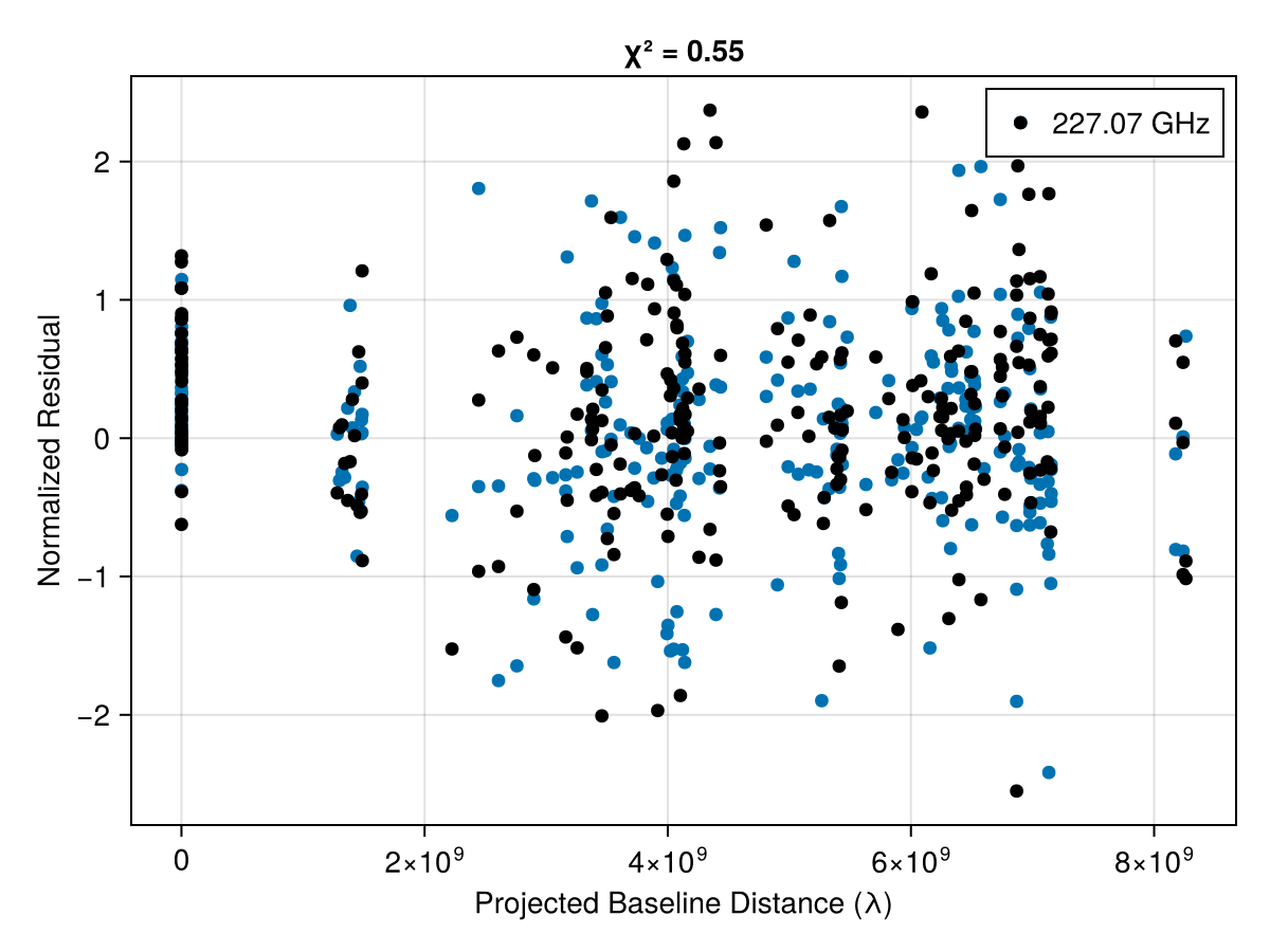
These look reasonable, although there may be some minor overfitting. This could be improved in a few ways, but that is beyond the goal of this quick tutorial. Plotting the image, we see that we have a much cleaner version of the closure-only image from Imaging a Black Hole using only Closure Quantities.
g = imagepixels(fovx, fovy, 128, 128)
img = intensitymap(skymodel(post, xopt), g)
imageviz(img, size = (500, 400)) |> DisplayAs.PNG |> DisplayAs.Text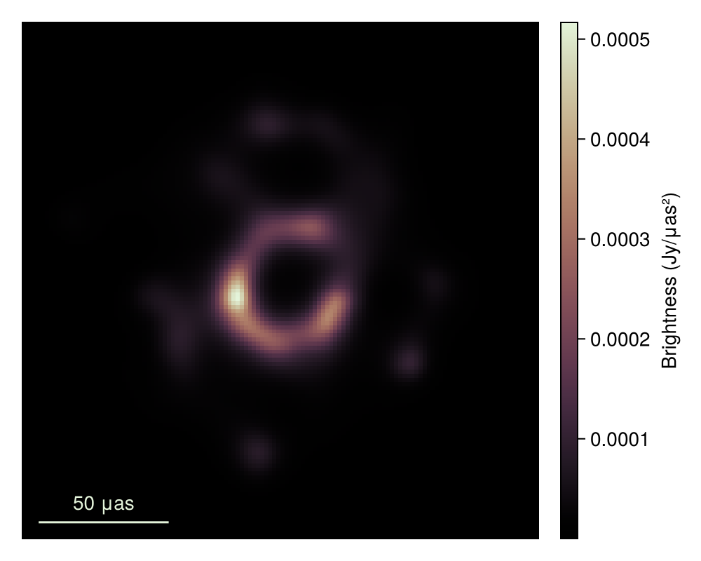
Because we also fit the instrument model, we can inspect their parameters. First, let's query the posterior object with the optimal parameters to get the instrument model.
intopt = instrumentmodel(post, xopt)126-element Comrade.SiteArray{ComplexF64, 1, Vector{ComplexF64}, Vector{Comrade.IntegrationTime{Int64, Float64}}, Vector{Comrade.FrequencyChannel{Float64, Int64}}, Vector{Symbol}}:
1.0516933592962758 + 0.0im
0.5423619644454115 + 0.9007439442386426im
0.986056814858046 + 0.0im
-0.6113897365930753 - 0.852703596798753im
-0.13090870517696226 + 0.7634862512662404im
0.7352274788447272 + 0.8794343862689954im
0.9944801955677527 + 0.0im
-0.6480172942029191 - 0.8143290744965743im
-0.18929860250750735 + 0.9209724363483106im
0.8514731503733395 + 0.6756637247362891im
1.00575913123764 + 0.0im
-0.6719233199584351 - 0.7861298432780356im
-0.1895911472820227 + 0.8640395977604969im
0.9277857103615266 + 0.490006761108028im
0.9781070679651204 + 0.0im
-0.7294458915721619 - 0.7684318452081814im
-0.22042719678236702 + 0.8797578775535361im
0.935862464627547 + 0.2786865284330235im
-0.7127672973858038 - 0.7508618471395395im
0.6637797747760737 - 0.019658024019063268im
0.8872134706782737 + 0.1330890606102374im
1.006021190819099 + 0.0im
-0.7647171013393042 - 0.6976080757696781im
-0.11985933578918527 + 0.5926978303513734im
0.979203240168178 - 0.0919992859560006im
0.9897103044518535 + 0.0im
-0.7925892247072904 - 0.6749374787396581im
-0.09932717113616225 + 0.5439578893340238im
0.9541136638182837 - 0.2944978090937636im
1.003284192518711 + 0.0im
-0.8077544189395781 - 0.6474532302412328im
-0.07451024943143392 + 0.5442153275368304im
0.8604014164315801 - 0.4922846818570326im
0.9843007521137929 + 0.0im
-0.8188938783814489 - 0.6505648806179837im
0.20836887830368409 + 0.9246036241082403im
-0.030716617319120294 + 0.4856756394217373im
0.7284575894560484 - 0.7113190186043599im
0.9720085308268425 + 0.0im
-0.8127911328145508 - 0.686672101124861im
0.34142713858989954 + 0.8581952611917072im
0.02095160196523166 + 0.5342102659806166im
0.5141295178547203 - 0.8452038448678617im
1.0163726572346896 + 0.0im
-0.8060354264392651 - 0.6439869971247174im
0.516740937547386 + 0.8164243759746683im
0.1118859918399041 + 0.6254332210970133im
0.315557557771683 - 1.0158423553633273im
0.9762319823187141 + 0.0im
-0.7610658537062774 - 0.739730733971166im
0.6677701192080875 + 0.702569469581384im
0.7280809736479593 - 0.7654487458371475im
0.16057259246808075 + 0.5411867607425936im
0.01629558630103451 - 1.106943515523204im
1.0217729637413282 + 0.0im
-0.7628158167333547 - 0.6658061664158446im
0.8221695961886637 + 0.5506133209512039im
0.8077804485299427 - 0.622733096496753im
0.24210842840592453 + 0.4870248966068455im
-0.3220228634107299 - 1.081335796751439im
-0.3279832003432633 - 0.9547586830117066im
0.9412268985960678 + 0.0im
-0.7922229435921258 - 0.7433222403700652im
0.9159561913763643 + 0.3905081691605497im
0.8605564970960189 - 0.5244590934601263im
0.30999860297028825 + 0.4003427583105817im
-0.6255074942438079 - 1.1179065272941222im
-0.5343771707907206 - 0.8566728874414826im
0.8747159106309785 + 0.0im
-0.7887796525075806 - 0.8766613976323547im
0.9657325131398458 + 0.23738317363696554im
0.9324572019307255 - 0.4177736196084151im
0.3954151371657948 + 0.3255022093683739im
-0.6461845018805097 - 0.7128128009153692im
-0.7426915706305044 - 0.7089710552778018im
0.9950792091561519 + 0.0im
1.0056508245383355 + 0.009102297120142197im
0.9638097619591908 - 0.3279675207087186im
0.4805751910771062 + 0.16841936883864864im
-0.8786522361790657 - 0.5106253806685549im
1.062098178894242 + 0.0im
-0.5966458049081486 - 0.7796138014091316im
0.9760539725768289 - 0.2853353903190754im
1.010127010770789 - 0.23988061141228215im
0.483894997248763 - 0.21738372793036406im
1.0201551447148842 + 0.0im
-0.5694128339533114 - 0.8443483741254795im
0.8879514029588459 - 0.47133774092853314im
0.997239811999705 - 0.19973544602291374im
0.20510357872337714 - 0.40276615693924206im
-0.9844639388400874 - 0.22997927912222887im
1.0913782344907916 + 0.0im
0.7449266033038227 - 0.7063206113059496im
1.006056336152552 - 0.1677862521221486im
0.019049101555803905 - 0.4809733087242452im
-1.0113107525577636 - 0.0842261662618931im
1.113103757592541 + 0.0im
-0.4779105246054072 - 0.800226023958167im
0.4990887138538776 - 0.8708653565604136im
1.005467138581833 - 0.15832946009928991im
-0.11496625851382096 - 0.39454663404405516im
-1.0100136106954354 + 0.0681525402018842im
1.0038119865904929 + 0.0im
-0.4397405564966201 - 0.9361714931496843im
0.27816396463530596 - 0.9742449713171101im
1.0044563506644613 - 0.15790219442386427im
-0.25160542562523375 - 0.3719577693161053im
-1.0107369202922278 + 0.13213004313356502im
0.9971858924480758 + 0.0im
-0.40729042289791373 - 0.9621672026825696im
0.034875721111129805 - 0.9937665415272818im
1.0026664990961884 - 0.1753071934167711im
-0.4100195783063915 - 0.40044454646725547im
-0.999993773174782 + 0.19344343871237069im
0.9681795095208777 + 0.0im
-0.3297371772200164 - 1.0054779254160522im
-0.1805089833513258 - 0.9597634206339444im
0.9945335961306364 - 0.2017347262649632im
-0.46766189745425224 - 0.31178410970223014im
-0.993253524211613 + 0.1841156187969254im
0.9858135223040104 + 0.0im
-0.26797015651677303 - 1.0181350543103431im
-0.2569036986933344 - 0.8769425045346487im
1.005172298363678 - 0.20848439118830472im
-0.4823167357169608 - 0.22936651343911016im
-0.9914404340791149 + 0.18944628121400722imThis returns a SiteArray object which contains the gains as a flat vector with metadata about the sites, time, and frequency. To visualize the gains we can use the plotcaltable function which automatically plots the gains. Since the gains are complex we will first plot the phases.
plotcaltable(angle.(intopt)) |> DisplayAs.PNG |> DisplayAs.Text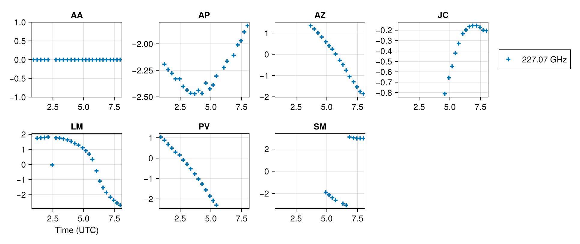
Due to the a priori calibration of the data, the gain phases are quite stable and just drift over time. Note that the one outlier around 2.5 UT is when ALMA leaves the array. As a result we shift the reference antenna to APEX on that scan causing the gain phases to jump.
We can also plot the gain amplitudes
plotcaltable(abs.(intopt)) |> DisplayAs.PNG |> DisplayAs.Text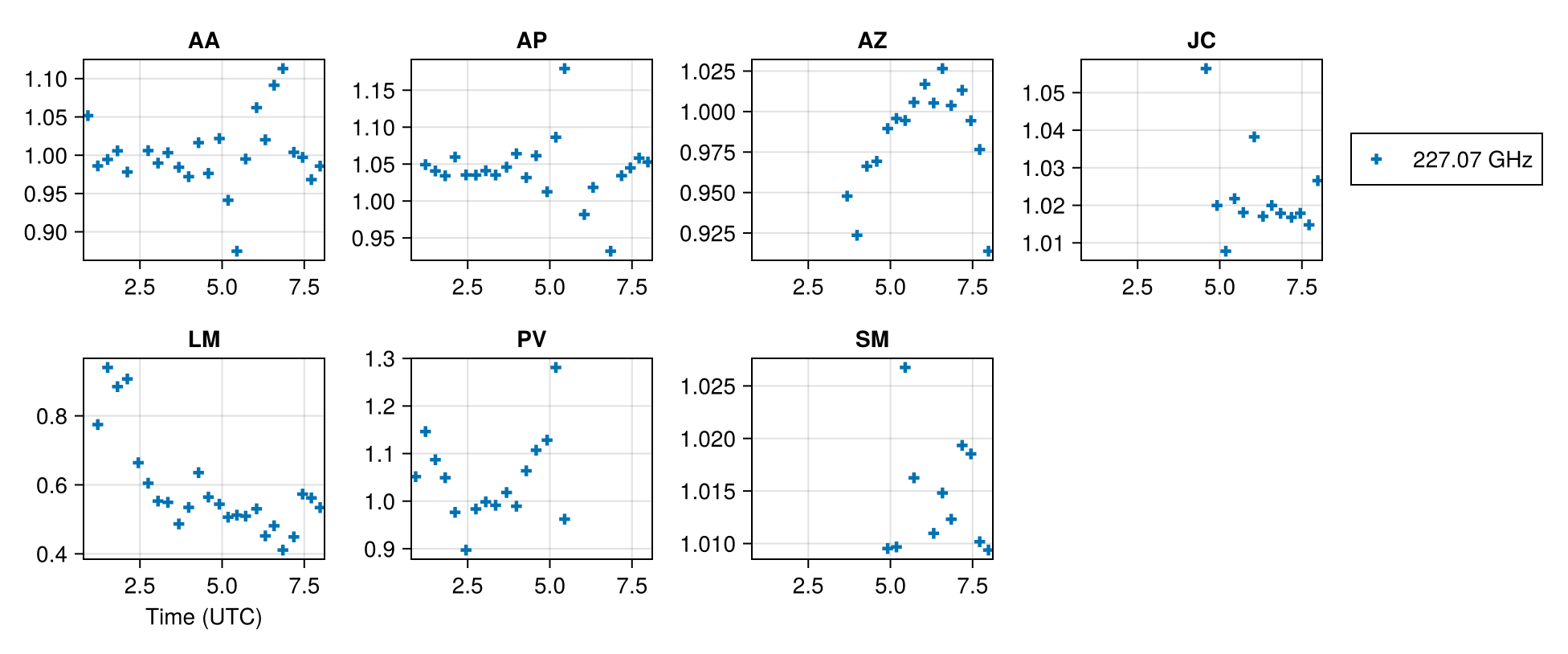
Here we find relatively stable gains for most stations. The exception is LMT which has a large offset after 2.5 UT. This is a known issue with the LMT in 2017 and is due to pointing issues. However, we can see the power of simultaneous imaging and instrument modeling as we are able to solve for the gain amplitudes and get a reasonable image.
Why we should Sample from the Posterior
One problem with the MAP estimate is that it does not provide uncertainties on the image. That is we are unable to statistically assess which components of the image are certain. Comrade is really a Bayesian imaging and calibration package for VLBI. Therefore, our goal is to sample from the posterior distribution of the image and instrument model. This is a very high-dimensional distribution with typically 1,000 - 100,000 parameters. To sample from this very high dimensional distribution, Comrade has an array of samplers that can be used. However, note that Comrade also satisfies the LogDensityProblems.jl interface. Therefore, you can use any package that supports LogDensityProblems.jl if you have your own fancy sampler.
For this example, we will use HMC, specifically the NUTS algorithm. For However, due to the need to sample a large number of gain parameters, constructing the posterior can take a few minutes. Therefore, for this tutorial, we will only do a quick preliminary run.
using AdvancedHMC
chain = sample(rng, post, NUTS(0.8), 700; n_adapts = 500, initial_params = xopt)
PosteriorSamples
Samples size: (700,)
sampler used: AHMC
Mean
┌───────────────────────────────────────────────────────────────────────────────
│ sky ⋯
│ @NamedTuple{c::@NamedTuple{params::Matrix{Float64}, hyperparams::Float64}, σ ⋯
├───────────────────────────────────────────────────────────────────────────────
│ (c = (params = [-0.00777631 0.0553803 … 0.0237059 -0.0177215; 0.0235398 0.06 ⋯
└───────────────────────────────────────────────────────────────────────────────
2 columns omitted
Std. Dev.
┌───────────────────────────────────────────────────────────────────────────────
│ sky ⋯
│ @NamedTuple{c::@NamedTuple{params::Matrix{Float64}, hyperparams::Float64}, σ ⋯
├───────────────────────────────────────────────────────────────────────────────
│ (c = (params = [0.539682 0.608198 … 0.563194 0.525407; 0.601253 0.651664 … 0 ⋯
└───────────────────────────────────────────────────────────────────────────────
2 columns omittedNote
The above sampler will store the samples in memory, i.e. RAM. For large models this can lead to out-of-memory issues. To avoid this we recommend using the saveto = DiskStore() kwargs which periodically saves the samples to disk limiting memory useage. You can load the chain using load_samples(diskout) where diskout is the object returned from sample.
Now we prune the adaptation phase
chain = chain[(begin + 500):end]PosteriorSamples
Samples size: (200,)
sampler used: AHMC
Mean
┌───────────────────────────────────────────────────────────────────────────────
│ sky ⋯
│ @NamedTuple{c::@NamedTuple{params::Matrix{Float64}, hyperparams::Float64}, σ ⋯
├───────────────────────────────────────────────────────────────────────────────
│ (c = (params = [-0.0102205 0.0422304 … 0.0406638 0.0775556; 0.00494859 0.076 ⋯
└───────────────────────────────────────────────────────────────────────────────
2 columns omitted
Std. Dev.
┌───────────────────────────────────────────────────────────────────────────────
│ sky ⋯
│ @NamedTuple{c::@NamedTuple{params::Matrix{Float64}, hyperparams::Float64}, σ ⋯
├───────────────────────────────────────────────────────────────────────────────
│ (c = (params = [0.598324 0.600126 … 0.538025 0.521172; 0.62907 0.646684 … 0. ⋯
└───────────────────────────────────────────────────────────────────────────────
2 columns omittedWarning
This should be run for likely an order of magnitude more steps to properly estimate expectations of the posterior
Now that we have our posterior, we can put error bars on all of our plots above. Let's start by finding the mean and standard deviation of the gain phases
mchain = Comrade.rmap(mean, chain);
schain = Comrade.rmap(std, chain);
Now we can use the measurements package to automatically plot everything with error bars. First we create a caltable the same way but making sure all of our variables have errors attached to them.
using Measurements
gmeas = instrumentmodel(post, (; instrument = map((x, y) -> Measurements.measurement.(x, y), mchain.instrument, schain.instrument)))
ctable_am = caltable(abs.(gmeas))
ctable_ph = caltable(angle.(gmeas))
┌─────────┬───────────────────┬─────────┬──────────────┬───────────┬────────────
│ Ti │ Fr │ AA │ AP │ AZ │ J ⋯
│ Any │ Any │ Any │ Any │ Any │ An ⋯
├─────────┼───────────────────┼─────────┼──────────────┼───────────┼────────────
│ 0.92 hr │ 227.070705664 GHz │ 0.0±0.0 │ missing │ missing │ missin ⋯
│ 1.22 hr │ 227.070705664 GHz │ 0.0±0.0 │ -2.194±0.018 │ missing │ missin ⋯
│ 1.52 hr │ 227.070705664 GHz │ 0.0±0.0 │ -2.241±0.019 │ missing │ missin ⋯
│ 1.82 hr │ 227.070705664 GHz │ 0.0±0.0 │ -2.277±0.017 │ missing │ missin ⋯
│ 2.12 hr │ 227.070705664 GHz │ 0.0±0.0 │ -2.329±0.017 │ missing │ missin ⋯
│ 2.45 hr │ 227.070705664 GHz │ missing │ -2.329±0.017 │ missing │ missin ⋯
│ 2.75 hr │ 227.070705664 GHz │ 0.0±0.0 │ -2.404±0.02 │ missing │ missin ⋯
│ 3.05 hr │ 227.070705664 GHz │ 0.0±0.0 │ -2.437±0.017 │ missing │ missin ⋯
│ 3.35 hr │ 227.070705664 GHz │ 0.0±0.0 │ -2.464±0.018 │ missing │ missin ⋯
│ 3.68 hr │ 227.070705664 GHz │ 0.0±0.0 │ -2.469±0.017 │ 1.51±0.38 │ missin ⋯
│ 3.98 hr │ 227.070705664 GHz │ 0.0±0.0 │ -2.44±0.018 │ 1.37±0.38 │ missin ⋯
│ 4.28 hr │ 227.070705664 GHz │ 0.0±0.0 │ -2.468±0.016 │ 1.19±0.38 │ missin ⋯
│ 4.58 hr │ 227.070705664 GHz │ 0.0±0.0 │ -2.371±0.019 │ 1.0±0.38 │ -0.48±0.3 ⋯
│ 4.92 hr │ 227.070705664 GHz │ 0.0±0.0 │ -2.422±0.02 │ 0.79±0.38 │ -0.34±0.3 ⋯
│ 5.18 hr │ 227.070705664 GHz │ 0.0±0.0 │ -2.386±0.017 │ 0.6±0.38 │ -0.25±0.3 ⋯
│ ⋮ │ ⋮ │ ⋮ │ ⋮ │ ⋮ │ ⋱
└─────────┴───────────────────┴─────────┴──────────────┴───────────┴────────────
4 columns and 10 rows omittedNow let's plot the phase curves
plotcaltable(ctable_ph) |> DisplayAs.PNG |> DisplayAs.Text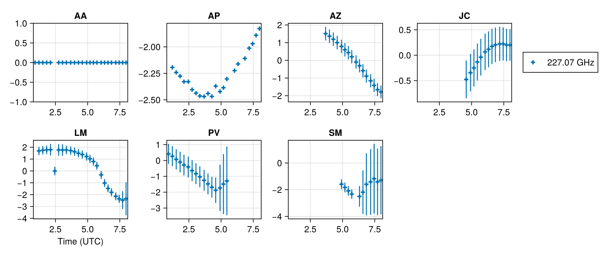
and now the amplitude curves
plotcaltable(ctable_am) |> DisplayAs.PNG |> DisplayAs.Text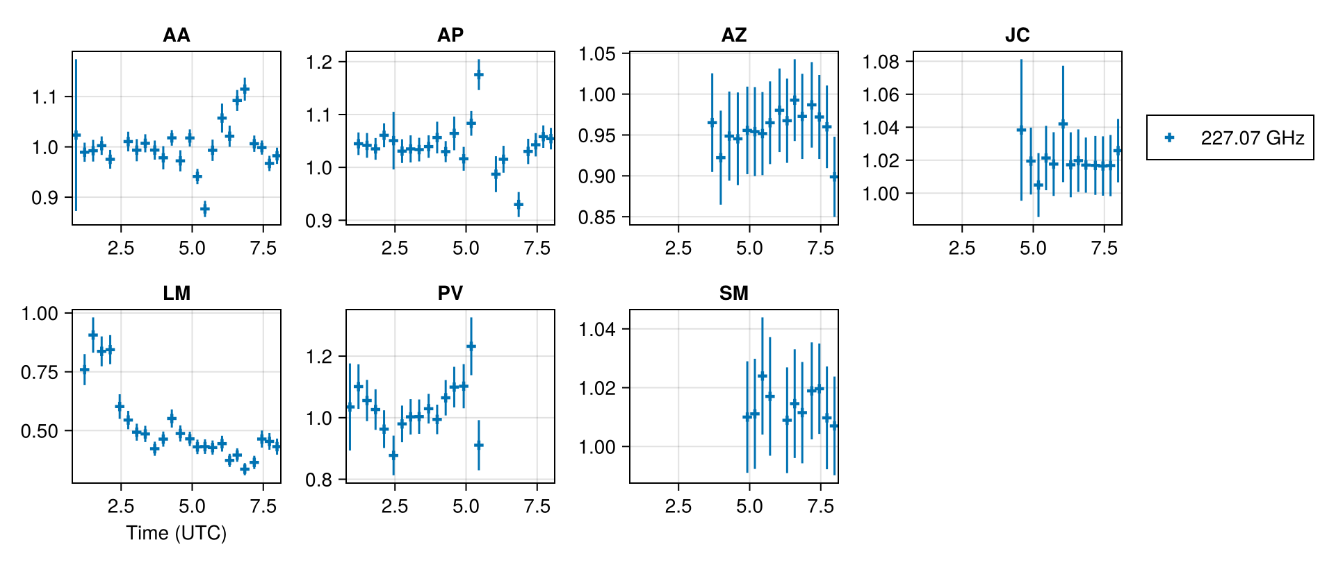
Finally let's construct some representative image reconstructions.
samples = skymodel.(Ref(post), chain[begin:5:end])
imgs = intensitymap.(samples, Ref(g))

mimg = mean(imgs)
simg = std(imgs)
fig = Figure(; size = (700, 700));
axs = [Axis(fig[i, j], xreversed = true, aspect = 1) for i in 1:2, j in 1:2]
image!(axs[1, 1], mimg, colormap = :afmhot); axs[1, 1].title = "Mean"
image!(axs[1, 2], simg ./ (max.(mimg, 1.0e-8)), colorrange = (0.0, 2.0), colormap = :afmhot);axs[1, 2].title = "Frac. Uncer."
image!(axs[2, 1], imgs[1], colormap = :afmhot);
image!(axs[2, 2], imgs[end], colormap = :afmhot);
hidedecorations!.(axs)
fig |> DisplayAs.PNG |> DisplayAs.Text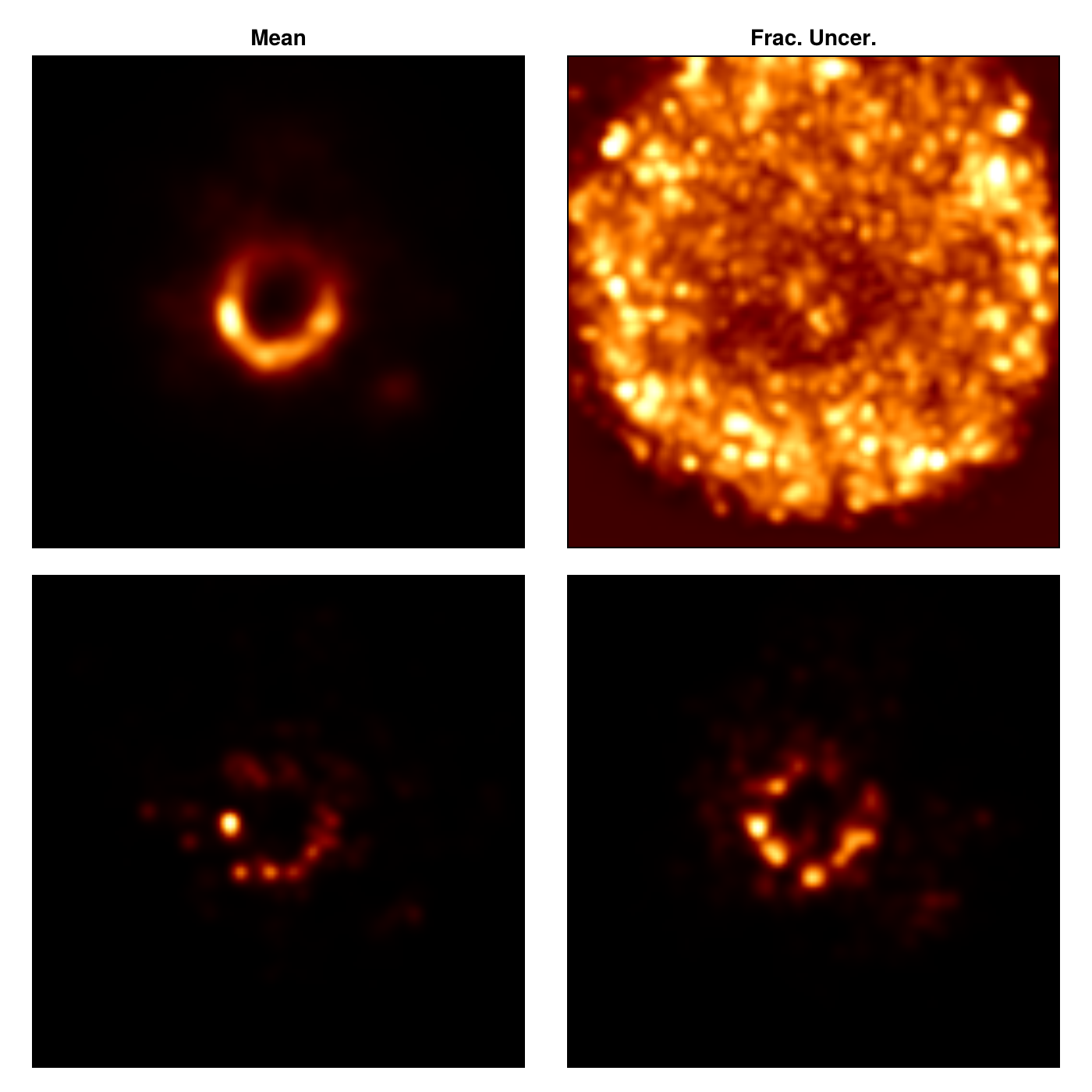
And viola, you have just finished making a preliminary image and instrument model reconstruction. In reality, you should run the sample step for many more MCMC steps to get a reliable estimate for the reconstructed image and instrument model parameters.
This page was generated using Literate.jl.