Loading Data into Comrade

The VLBI field does not have a standardized data format, and the EHT uses a particular uvfits format similar to the optical interferometry oifits format. As a result, we reuse the excellent eht-imaging package to load data into Comrade.

Once the data is loaded, we then convert the data into the tabular format Comrade expects. Note that this may change to a Julia package as the Julia radio astronomy group grows.

To get started, we will load Comrade and Plots to enable visualizations of the data

using Comrade

using Plots

We also load Pyehtim since it loads eht-imaging into Julia using PythonCall and exports the variable ehtim

using Pyehtim

To load the data we will use eht-imaging. We will use the 2017 public M87 data which can be downloaded from cyverse

obseht = ehtim.obsdata.load_uvfits(joinpath(__DIR, "..", "..", "Data", "SR1_M87_2017_096_lo_hops_netcal_StokesI.uvfits"))

Python: <ehtim.obsdata.Obsdata object at 0x7fafb20465c0>

Now we will average the data over telescope scans. Note that the EHT data has been pre-calibrated so this averaging doesn't induce large coherence losses.

obs = Pyehtim.scan_average(obseht)

Python: <ehtim.obsdata.Obsdata object at 0x7fafce115720>

Warning

We use a custom scan-averaging function to ensure that the scan-times are homogenized.

We can now extract data products that Comrade can use

vis    = extract_table(obs, Visibilities()) ## complex visibilites
amp    = extract_table(obs, VisibilityAmplitudes()) ## visibility amplitudes
cphase = extract_table(obs, ClosurePhases(; snrcut=3.0)) ## extract minimal set of closure phases
lcamp  = extract_table(obs, LogClosureAmplitudes(; snrcut=3.0)) ## extract minimal set of log-closure amplitudes

EHTObservationTable{Comrade.EHTLogClosureAmplitudeDatum{:I}}
  source:      M87
  mjd:         57849
  bandwidth:   1.856e9
  sites:       [:AA, :AP, :AZ, :JC, :LM, :PV, :SM]
  nsamples:    129

For polarization we first load the data in the cirular polarization basis Additionally, we load the array table at the same time to load the telescope mounts.

obseht = Pyehtim.load_uvfits_and_array(
                joinpath(__DIR, "..", "..", "Data", "polarized_gaussian_all_corruptions.uvfits"),
                joinpath(__DIR, "..", "..", "Data", "array.txt"),
                polrep="circ"
                        )
obs = Pyehtim.scan_average(obseht)
coh = extract_table(obs, Coherencies())

EHTObservationTable{Comrade.EHTCoherencyDatum{Float64}}
  source:      17.761122472222223:-28.992189444444445
  mjd:         51544
  bandwidth:   1.0e9
  sites:       [:AA, :AP, :AZ, :JC, :LM, :PV, :SM]
  nsamples:    315

Warning

Always use our extract_cphase and extract_lcamp functions to find the closures eht-imaging will sometimes incorrectly calculate a non-redundant set of closures.

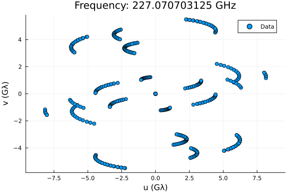
We can also recover the array used in the observation using

using DisplayAs
ac = arrayconfig(vis)
plot(ac) |> DisplayAs.PNG |> DisplayAs.Text # Plot the baseline coverage

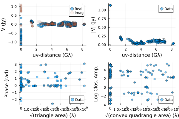
To plot the data we just call

l = @layout [a b; c d]
pv = plot(vis);
pa = plot(amp);
pcp = plot(cphase);
plc = plot(lcamp);
plot(pv, pa, pcp, plc; layout=l) |> DisplayAs.PNG |> DisplayAs.Text

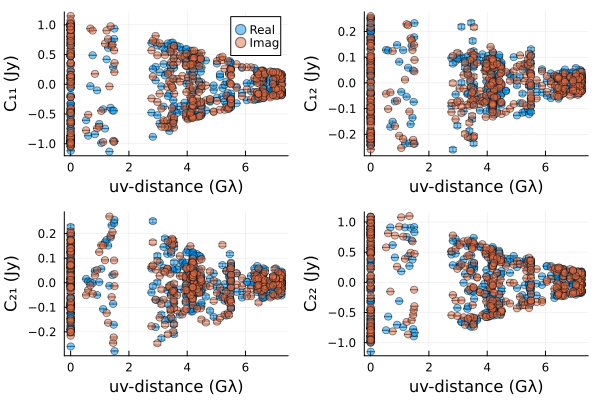
And also the coherency matrices

plot(coh) |> DisplayAs.PNG |> DisplayAs.Text

---

This page was generated using Literate.jl.