Polarized Image and Instrumental Modeling

In this tutorial, we will analyze a simulated simple polarized dataset to demonstrate Comrade's polarized imaging capabilities.

Introduction to Polarized Imaging

The EHT is a polarized interferometer. However, like all VLBI interferometers, it does not directly measure the Stokes parameters (I, Q, U, V). Instead, it measures components related to the electric field at the telescope along two directions using feeds. There are two types of feeds at telescopes: circular, which measure $R / L$ components of the electric field, and linear feeds, which measure $X / Y$ components of the electric field. Most sites in the EHT use circular feeds, meaning they measure the right (R) and left electric field (L) at each telescope. Although note that ALMA actually uses linear feeds. Currently Comrade has the ability to fit natively mixed polarization data however, the publically released EHT data has been converted to circular polarization. For a VLBI array whose feeds are purely circluar the coherency matrices are given by,

C_{i j} = (\begin{matrix} R R^{*} & R L^{*} \\ L R^{*} & L L^{*} \end{matrix}) .

These coherency matrices are the fundamental object in interferometry and what the telescope observes. For a perfect interferometer, these circular coherency matrices are related to the usual Fourier transform of the stokes parameters by

(\begin{matrix} \tilde{I} \\ \tilde{Q} \\ \tilde{U} \\ \tilde{V} \end{matrix}) = \frac{1}{2} (\begin{matrix} R R^{*} + L L^{*} \\ R L^{*} + L R^{*} \\ i (L R^{*} - R L^{*}) \\ R R^{*} - L L^{*} \end{matrix}) .

Note

In this tutorial, we stick to circular feeds but Comrade has the capabilities to model linear (XX,XY, ...) and mixed basis coherencies (e.g., RX, RY, ...).

In reality, the measure coherencies are corrupted by both the atmosphere and the telescope itself. In Comrade we use the RIME formalism ^[1] to represent these corruptions, namely our measured coherency matrices $V_{i j}$ are given by

V_{i j} = J_{i} C_{i j} J_{j}^{†}

where $J$ is known as a Jones matrix and $i j$ denotes the baseline $i j$ with sites $i$ and $j$ .

Comrade is highly flexible with how the Jones matrices are formed and provides several convenience functions that parameterize standard Jones matrices. These matrices include:

JonesG which builds the set of complex gain Jones matrices

G = (\begin{matrix} g_{a} & 0 \\ 0 & g_{b} \end{matrix})

JonesD which builds the set of complex d-terms Jones matrices

D = (\begin{matrix} 1 & d_{a} \\ d_{b} & 1 \end{matrix})

JonesR is the basis transform matrix $T$ . This transformation is special and combines two things using the decomposition $T = F B$ . The first, $B$ , is the transformation from some reference basis to the observed coherency basis (this allows for mixed basis measurements). The second is the feed rotation, $F$ , that transforms from some reference axis to the axis of the telescope as the source moves in the sky. The feed rotation matrix F for circular feeds in terms of the per station feed rotation angle $φ$ is

F = (\begin{matrix} e^{- i φ} & 0 \\ 0 & e^{i φ} \end{matrix})

In the rest of the tutorial, we are going to solve for all of these instrument model terms on in addition to our image structure to reconstruct a polarized image of a synthetic dataset.

Load the Data

To get started we will load Comrade

julia

using Comrade

Load the Data

julia

using Pyehtim

For reproducibility we use a stable random number genreator

julia

using StableRNGs
rng = StableRNG(42)

StableRNGs.LehmerRNG(state=0x00000000000000000000000000000055)

Now we will load some synthetic polarized data.

julia

obs = Pyehtim.load_uvfits_and_array(
        joinpath(__DIR, "..", "..", "Data", "polarized_gaussian_all_corruptions.uvfits"),
        joinpath(__DIR, "..", "..", "Data", "array.txt"), polrep="circ")

Python: <ehtim.obsdata.Obsdata object at 0x7faf3ae878e0>

Notice that, unlike other non-polarized tutorials, we need to include a second argument. This is the array file of the observation and is required to determine the feed rotation of the array.

Now we scan average the data since the data to boost the SNR and reduce the total data volume.

julia

obs = scan_average(obs)

Python: <ehtim.obsdata.Obsdata object at 0x7fafc0b9b250>

Now we extract our observed/corrupted coherency matrices.

julia

dvis = extract_table(obs, Coherencies())

EHTObservationTable{Comrade.EHTCoherencyDatum{Float64}}
  source:      17.761122472222223:-28.992189444444445
  mjd:         51544
  bandwidth:   1.0e9
  sites:       [:AA, :AP, :AZ, :JC, :LM, :PV, :SM]
  nsamples:    315

##Building the Model/Posterior

To build the model, we first break it down into two parts:

The image or sky model. In Comrade, all polarized image models are written in terms of the Stokes parameters. In this tutorial, we will use a polarized image model based on Pesce (2021)^[2], and parameterizes each pixel in terms of the Poincare sphere. This parameterization ensures that we have all the physical properties of stokes parameters. Note that we also have a parameterization in terms of hyperbolic trig functions VLBISkyModels.PolExp2Map
The instrument model. The instrument model specifies the model that describes the impact of instrumental and atmospheric effects. We will be using the $J = G D R$ decomposition we described above. However, to parameterize the R/L complex gains, we will be using a gain product and ratio decomposition. The reason for this decomposition is that in realistic measurements, the gain ratios and products have different temporal characteristics. Namely, many of the EHT observations tend to demonstrate constant R/L gain ratios across an nights observations, compared to the gain products, which vary every scan. Additionally, the gain ratios tend to be smaller (i.e., closer to unity) than the gain products. Using this apriori knowledge, we can build this into our model and reduce the total number of parameters we need to model.

First we specify our sky model. As always Comrade requires this to be a two argument function where the first argument is typically a NamedTuple of parameters we will fit and the second are additional metadata required to build the model.

julia

using StatsFuns: logistic
function sky(θ, metadata)
    (;c, σ, p, p0, pσ, angparams) = θ
    (;ftot, grid) = metadata
    # Build the stokes I model
    rast = ftot*to_simplex(CenteredLR(), σ.*c.params)
    # The total polarization fraction is modeled in logit space so we transform it back
    pim = logistic.(p0 .+ pσ.*p.params)
    # Build our IntensityMap
    pmap = PoincareSphere2Map(rast, pim, angparams, grid)
    # Construct the actual image model which uses a third order B-spline pulse
    m = ContinuousImage(pmap, BSplinePulse{3}())
    # Finally find the image centroid and shift it to be at the center
    x0, y0 = centroid(pmap)
    ms = shifted(m, -x0, -y0)
    return ms
end

sky (generic function with 1 method)

Now, we define the model metadata required to build the model. We specify our image grid and cache model needed to define the polarimetric image model. Our image will be a 10x10 raster with a 60μas FOV.

julia

using Distributions, DistributionsAD
using VLBIImagePriors
fovx = μas2rad(60.0)
fovy = μas2rad(60.0)
nx = ny = 10
grid = imagepixels(fovx, fovy, nx, ny)

RectiGrid(
executor: Serial()
Dimensions: 
↓ X Sampled{Float64} LinRange{Float64}(-1.3089969389957472e-10, 1.3089969389957472e-10, 10) ForwardOrdered Regular Points,
→ Y Sampled{Float64} LinRange{Float64}(-1.3089969389957472e-10, 1.3089969389957472e-10, 10) ForwardOrdered Regular Points
)

For the image metadata we specify the grid and the total flux of the image, which is 1.0. Note that we specify the total flux out front since it is degenerate with an overall shift in the gain amplitudes.

julia

skymeta = (;ftot=1.0, grid)

(ftot = 1.0, grid = RectiGrid{Tuple{X{DimensionalData.Dimensions.Lookups.Sampled{Float64, LinRange{Float64, Int64}, DimensionalData.Dimensions.Lookups.ForwardOrdered, DimensionalData.Dimensions.Lookups.Regular{Float64}, DimensionalData.Dimensions.Lookups.Points, DimensionalData.Dimensions.Lookups.NoMetadata}}, Y{DimensionalData.Dimensions.Lookups.Sampled{Float64, LinRange{Float64, Int64}, DimensionalData.Dimensions.Lookups.ForwardOrdered, DimensionalData.Dimensions.Lookups.Regular{Float64}, DimensionalData.Dimensions.Lookups.Points, DimensionalData.Dimensions.Lookups.NoMetadata}}}, Serial, ComradeBase.NoHeader}((X{DimensionalData.Dimensions.Lookups.Sampled{Float64, LinRange{Float64, Int64}, DimensionalData.Dimensions.Lookups.ForwardOrdered, DimensionalData.Dimensions.Lookups.Regular{Float64}, DimensionalData.Dimensions.Lookups.Points, DimensionalData.Dimensions.Lookups.NoMetadata}}([-1.3089969389957472e-10, -1.0181087303300256e-10, -7.27220521664304e-11, -4.363323129985825e-11, -1.454441043328608e-11, 1.454441043328608e-11, 4.363323129985823e-11, 7.27220521664304e-11, 1.0181087303300256e-10, 1.3089969389957472e-10]), Y{DimensionalData.Dimensions.Lookups.Sampled{Float64, LinRange{Float64, Int64}, DimensionalData.Dimensions.Lookups.ForwardOrdered, DimensionalData.Dimensions.Lookups.Regular{Float64}, DimensionalData.Dimensions.Lookups.Points, DimensionalData.Dimensions.Lookups.NoMetadata}}([-1.3089969389957472e-10, -1.0181087303300256e-10, -7.27220521664304e-11, -4.363323129985825e-11, -1.454441043328608e-11, 1.454441043328608e-11, 4.363323129985823e-11, 7.27220521664304e-11, 1.0181087303300256e-10, 1.3089969389957472e-10])), Serial(), ComradeBase.NoHeader()))

For our image prior we will use a simpler prior than

We use again use a GMRF prior. For more information see the Imaging a Black Hole using only Closure Quantities tutorial.
For the total polarization fraction, p, we assume an uncorrelated uniform prior ImageUniform for each pixel.
To specify the orientation of the polarization, angparams, on the Poincare sphere, we use a uniform spherical distribution, ImageSphericalUniform.

julia

rat = beamsize(dvis)/step(grid.X)
cmarkov = ConditionalMarkov(GMRF, grid; order=1)
dρ = truncated(InverseGamma(1.0, -log(0.1)*rat); lower=2.0, upper=max(nx, ny))
cprior = HierarchicalPrior(cmarkov, dρ)

HierarchicalPrior(
	map: 
	ConditionalMarkov(
Random Field: GaussMarkovRandomField
Graph: MarkovRandomFieldGraph{1}(
dims: (10, 10)
)
)	hyper prior: 
	Truncated(Distributions.InverseGamma{Float64}(
invd: Distributions.Gamma{Float64}(α=1.0, θ=0.09157612316984907)
θ: 10.919876987424647
)
; lower=2.0, upper=10.0)

)

For all the calibration parameters, we use a helper function CalPrior which builds the prior given the named tuple of station priors and a JonesCache that specifies the segmentation scheme. For the gain products, we use the scancache, while for every other quantity, we use the trackcache.

julia

fwhmfac = 2.0*sqrt(2.0*log(2.0))
skyprior = (
    c = cprior,
    σ  = truncated(Normal(0.0, 1.0); lower=0.0),
    p  = cprior,
    p0 = Normal(-2.0, 2.0),
    pσ =  truncated(Normal(0.0, 1.0); lower=0.01),
    angparams = ImageSphericalUniform(nx, ny),
    )

skym = SkyModel(sky, skyprior, grid; metadata=skymeta)

 SkyModel
  with map: sky
   on grid: RectiGrid

Now we build the instrument model. Due to the complexity of VLBI the instrument model is critical to the success of imaging and getting reliable results. For this example we will use the standard instrument model used in polarized EHT analyses expressed in the RIME formalism. Our Jones decomposition will be given by GDR, where G are the complex gains, D are the d-terms, and R is what we call the ideal instrument response, which is how an ideal interferometer using the feed basis we observe relative to some reference basis.

Given the possible flexibility in different parameterizations of the individual Jones matrices each Jones matrix requires the user to specify a function that converts from parameters to specific parameterization f the jones matrices.

For the complex gain matrix, we used the JonesG jones matrix. The first argument is now a function that converts from the parameters to the complex gain matrix. In this case, we will use a amplitude and phase decomposition of the complex gain matrix. Note that since the gain matrix is a diagonal 2x2 matrix the function must return a 2-element tuple. The first element of the tuple is the gain for the first polarization feed (R) and the second is the gain for the second polarization feed (L).

julia

G = JonesG() do x
    gR = exp(x.lgR + 1im*x.gpR)
    gL = gR*exp(x.lgrat + 1im*x.gprat)
    return gR, gL
end

JonesG{Main.var"#1#2"}(Main.var"#1#2"())

Note that we are using the Julia do syntax here to define an anonymous function. This could've also been written as

julia

fgain(x) = (exp(x.lgR + 1im*x.gpR), exp(x.lgR + x.lgrat + 1im*(x.gpR + x.gprat)))
G = JonesG(fgain)

Similarly we provide a JonesD function for the leakage terms. Since we assume that we are in the small leakage limit, we will use the decomposition 1 d1 d2 1 Therefore, there are 2 free parameters for the JonesD our parameterization function must return a 2-element tuple. For d-terms we will use a re-im parameterization.

julia

D = JonesD() do x
    dR = complex(x.dRx, x.dRy)
    dL = complex(x.dLx, x.dLy)
    return dR, dL
end

JonesD{Main.var"#3#4"}(Main.var"#3#4"())

Finally we define our response Jones matrix. This matrix is a basis transform matrix plus the feed rotation angle for each station. These are typically set by the telescope so there are no free parameters, so no parameterization is necessary.

julia

R = JonesR(;add_fr=true)

JonesR{Nothing}(nothing, true)

Finally, we build our total Jones matrix by using the JonesSandwich function. The first argument is a function that specifies how to combine each Jones matrix. In this case, we are completely standard so we just need to multiply the different jones matrices. Note that if no function is provided, the default is to multiply the Jones matrices, so we could've removed the * argument in this case.

julia

J = JonesSandwich(splat(*), G, D, R)


intprior = (
    lgR  = ArrayPrior(IIDSitePrior(ScanSeg(), Normal(0.0, 0.1))),
    gpR  = ArrayPrior(IIDSitePrior(ScanSeg(), DiagonalVonMises(0.0, inv(π  ^2))); refant=SEFDReference(0.0), phase=false),
    lgrat= ArrayPrior(IIDSitePrior(ScanSeg(), Normal(0.0, 0.1)), phase=true),
    gprat= ArrayPrior(IIDSitePrior(ScanSeg(), Normal(0.0, 0.1)); refant = SingleReference(:AA, 0.0)),
    dRx  = ArrayPrior(IIDSitePrior(TrackSeg(), Normal(0.0, 0.2))),
    dRy  = ArrayPrior(IIDSitePrior(TrackSeg(), Normal(0.0, 0.2))),
    dLx  = ArrayPrior(IIDSitePrior(TrackSeg(), Normal(0.0, 0.2))),
    dLy  = ArrayPrior(IIDSitePrior(TrackSeg(), Normal(0.0, 0.2))),
)

intmodel = InstrumentModel(J, intprior)

InstrumentModel
  with Jones:  JonesSandwich
  with reference basis: CirBasis()

Putting it all together, we form our likelihood and posterior objects for optimization and sampling.

julia

post = VLBIPosterior(skym, intmodel, dvis)

VLBIPosterior
ObservedSkyModel
  with map: sky
   on grid: FourierDualDomainObservedInstrumentModel
  with Jones:  JonesSandwich
  with reference basis: CirBasis()Data Products: Comrade.EHTCoherencyDatum

Reconstructing the Image and Instrument Effects

To sample from this posterior, it is convenient to move from our constrained parameter space to an unconstrained one (i.e., the support of the transformed posterior is (-∞, ∞)). This transformation is done using the asflat function.

julia

tpost = asflat(post)

TransformedVLBIPosterior(
VLBIPosterior
ObservedSkyModel
  with map: sky
   on grid: FourierDualDomainObservedInstrumentModel
  with Jones:  JonesSandwich
  with reference basis: CirBasis()Data Products: Comrade.EHTCoherencyDatum
Transform: Params to ℝ^1329
)

We can also query the dimension of our posterior or the number of parameters we will sample.

Warning

This can often be different from what you would expect. This difference is especially true when using angular variables, where we often artificially increase the dimension of the parameter space to make sampling easier.

julia

ndim = dimension(tpost)

Now we optimize. Unlike other imaging examples, we move straight to gradient optimizers due to the higher dimension of the space. In addition the only AD package that can currently work with the polarized Comrade posterior is Zygote. Note that in the future we expect to shift entirely to Enzyme, and in fact large portions of Comrade's AD already uses Enzyme through custom rules.

julia

using Optimization
using OptimizationOptimisers
using Zygote
xopt, sol = comrade_opt(post, Optimisers.Adam(), Optimization.AutoZygote(); initial_params=prior_sample(rng, post), maxiters=20_000)

((sky = (c = (params = [0.5355522693776443 0.29246414947259364 … -0.44227817107962153 1.2863900519659541; 1.0216116893032372 2.3043851761678398 … -0.637013120460028 -0.038207264389283534; … ; 0.9562912227194387 -0.22105432519182844 … 0.27794229430387296 1.1738028691524434; -0.22979945808700472 -0.10692735732948239 … -0.38300506825357244 0.6795242013019732], hyperparams = 6.7400727698666145), σ = 2.5476711341847325, p = (params = [0.23634931920533722 0.40190718856882995 … 0.14588670145393318 -0.21516782615666089; 0.5350370900231958 -0.1309999464396134 … 0.21569569840548883 0.038857440462085405; … ; 0.15514364067828493 0.24960915195430303 … 0.21849321428058113 -0.21286088693015698; 0.2589014724681644 0.3421128519466939 … 0.14836841094450573 0.035846120018505984], hyperparams = 3.8754795386304908), p0 = -0.9695842573272795, pσ = 3.9067726043626902, angparams = ([0.7182328967909022 -0.29842822136170877 … -0.7513156308168648 -0.23817112942680624; -0.11453436562669074 0.03292105443662291 … -0.3606177195191312 0.8680634712444172; … ; 0.020864799418456426 0.7152847052803837 … -0.4818189057707221 -0.315955773847622; 0.6056649881874611 0.6198248077353072 … -0.22208119707159182 0.18548748461347464], [0.42567060250392513 0.484295306385152 … 0.26223455177836286 0.9437852584090037; -0.9903173478709519 0.9158728017001552 … -0.8206653695820542 0.4709504071633839; … ; 0.9906799116287152 -0.29432007453621795 … -0.6250991669071989 0.7499105735192496; -0.7724428306276315 -0.7299041681852374 … -0.36802977567398065 0.40400017317455933], [0.5504053452968045 -0.8224345888325701 … 0.605605368820206 0.22922456045853717; -0.07844379896674748 0.4001165021349269 … 0.4432417078046378 0.1570717157343597; … ; -0.1346030194332534 0.6338323785646721 … -0.6140859659476269 -0.5812108745510361; -0.1910549541253891 0.2881963097989042 … -0.902903110042605 0.8957556883027269])), instrument = (lgR = [-0.037234314307177135, -0.03723431430243405, -0.0286567166900901, -0.028656716498255266, -0.05410063473582679, -0.054100634692400215, -0.04855143231996311, -0.04855143228122844, 0.006736870007627267, 0.006736869839255871  …  -0.026697458414928214, -0.026697458415177164, -0.01051946651991402, -0.010519466519836245, -0.005637454444155033, -0.005637454443959899, 0.005971613348054574, 0.0059716133905360225, -0.01045243044083296, -0.010452430439695107], gpR = [0.0, 2.207499792269091, 0.0, -0.7286000561118833, 0.0, -1.7176741615364814, 0.0, 1.1655662124910178, 0.0, 0.9175715612096428  …  0.0, -0.7103546214945599, 0.0, 3.078599322329672, 0.0, -1.7081957582310614, 0.0, -2.4545942007265316, 0.0, 2.9066966108215473], lgrat = [0.0319533967003419, 0.0044928550688850405, 0.06188392520943233, -0.0314733841850398, 0.015632301956316257, 0.018615113001226896, 0.05899451118524142, -0.02046224596193781, 0.07355882750126395, -0.03597561981343664  …  0.06059135185260098, -0.011283015789580554, 0.04077148357427639, 0.01208465618333324, 0.003731106092714386, 0.04261730385468398, -0.010076823560697765, 0.05625285734809124, 0.009287195520667542, 0.03391953804330737], gprat = [-0.0282385540330643, -0.00598921415952569, -0.11600217905935167, -0.22986731786907363, 0.19337715868644692, -0.11333477682909271, 0.050860354032374065, 0.013661800345647734, -0.11370711202669745, 0.0200625413391634  …  -0.10438018594084357, 0.0776379669885795, 0.14470796387357454, 0.020403302465553417, -0.001815553229860301, -0.13552482150179973, -0.12459883903805989, -0.03227361977550289, 0.0997292892786674, 0.10357486109014263], dRx = [0.010184691291046226, -0.0814438110007884, 0.09181356528450493, -0.042959995452969746, 0.030908549646163984, -0.007080029556868393, 0.07970343723198939], dRy = [-0.020027819701128127, 0.07150687653867778, -0.10164512224326394, 0.04966012557741396, -0.020434865487649626, 0.018211338447415806, -0.07103824636056831], dLx = [0.029289872489520058, -0.058604669609265324, 0.0887826485756546, -0.05867711375688718, 0.009856469699029632, -0.023993028435418225, 0.058895036739103034], dLy = [-0.0392239348044343, 0.04876562492068198, -0.078521300131849, 0.06878142601019495, -0.0002947675818690222, 0.039621595718056325, -0.05188050683197765])), retcode: Default
u: [0.5355522693776443, 1.0216116893032372, 2.479091094190481, 2.349928162071704, 2.2873417841678303, 2.16995145755935, -0.005644287391759657, 0.09241928679591821, 0.9562912227194387, -0.22979945808700472  …  0.009856469699029632, -0.023993028435418225, 0.058895036739103034, -0.0392239348044343, 0.04876562492068198, -0.078521300131849, 0.06878142601019495, -0.0002947675818690222, 0.039621595718056325, -0.05188050683197765]
Final objective value:     1232.3894692958763
)

Warning

Fitting polarized images is generally much harder than Stokes I imaging. This difficulty means that optimization can take a long time, and starting from a good starting location is often required.

Now let's evaluate our fits by plotting the residuals

julia

using Plots
residual(post, xopt)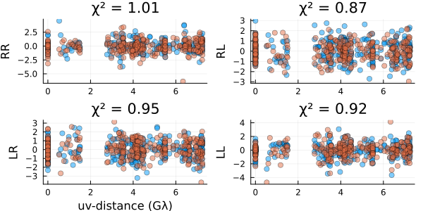

These look reasonable, although there may be some minor overfitting. Let's compare our results to the ground truth values we know in this example. First, we will load the polarized truth

julia

imgtrue = Comrade.load(joinpath(__DIR, "..", "..", "Data", "polarized_gaussian.fits"), IntensityMap{StokesParams})

╭─────────────────────────────────────────────────╮
│ 1024×1024 IntensityMap{StokesParams{Float64},2} │
├─────────────────────────────────────────────────┴────────────────────── dims ┐
  ↓ X Sampled{Float64} LinRange{Float64}(-4.843402302490755e-10, 4.843402302490755e-10, 1024) ForwardOrdered Regular Points,
  → Y Sampled{Float64} LinRange{Float64}(-4.843402302490772e-10, 4.843402302490772e-10, 1024) ForwardOrdered Regular Points
├──────────────────────────────────────────────────────────────────── metadata ┤
  ComradeBase.MinimalHeader{Float64}("SgrA", 266.4168370833333, -28.99218944444445, 51544.0, 2.3e11)
└──────────────────────────────────────────────────────────────────────────────┘
  ↓ →          …  4.8434e-10
 -4.8434e-10       [6.86545e-65, 4.08459e-78, 1.02982e-65, 1.02982e-66]
 -4.83393e-10      [8.99558e-65, 5.35191e-78, 1.34934e-65, 1.34934e-66]
 -4.82446e-10      [1.17804e-64, 7.00873e-78, 1.76706e-65, 1.76706e-66]
  ⋮            ⋱  
  4.82446e-10      [1.17804e-64, 7.00873e-78, 1.76706e-65, 1.76706e-66]
  4.83393e-10      [8.99558e-65, 5.35191e-78, 1.34934e-65, 1.34934e-66]
  4.8434e-10       [6.86545e-65, 4.08459e-78, 1.02982e-65, 1.02982e-66]

Select a reasonable zoom in of the image.

julia

imgtruesub = regrid(imgtrue, imagepixels(fovx, fovy, nx*4, ny*4))
img = intensitymap(Comrade.skymodel(post, xopt), axisdims(imgtruesub))

#Plotting the results gives
import CairoMakie as CM
using DisplayAs
fig = CM.Figure(;size=(450, 350));
axs = [CM.Axis(fig[1, i], xreversed=true, aspect=1) for i in 1:2]
polimage!(axs[1], imgtruesub,
                   nvec = 8,
                   length_norm=1/2, plot_total=true, pcolormap=:RdBu,
                   pcolorrange=(-0.25, 0.25),); axs[1].title="True"
polimage!(axs[2], img,
                   nvec = 8,
                   length_norm=1/2, plot_total=true, pcolormap=:RdBu,
                   pcolorrange=(-0.25, 0.25),);axs[2].title="Recon."
CM.Colorbar(fig[2,:], colormap=:RdBu, vertical=false, colorrange=(-0.25, 0.25), label="Signed Polarization Fraction sign(V)*|p|", flipaxis=false)
CM.colgap!(fig.layout, 3)
CM.rowgap!(fig.layout, 3)
CM.hidedecorations!.(fig.content[1:2])
fig |> DisplayAs.PNG |> DisplayAs.Text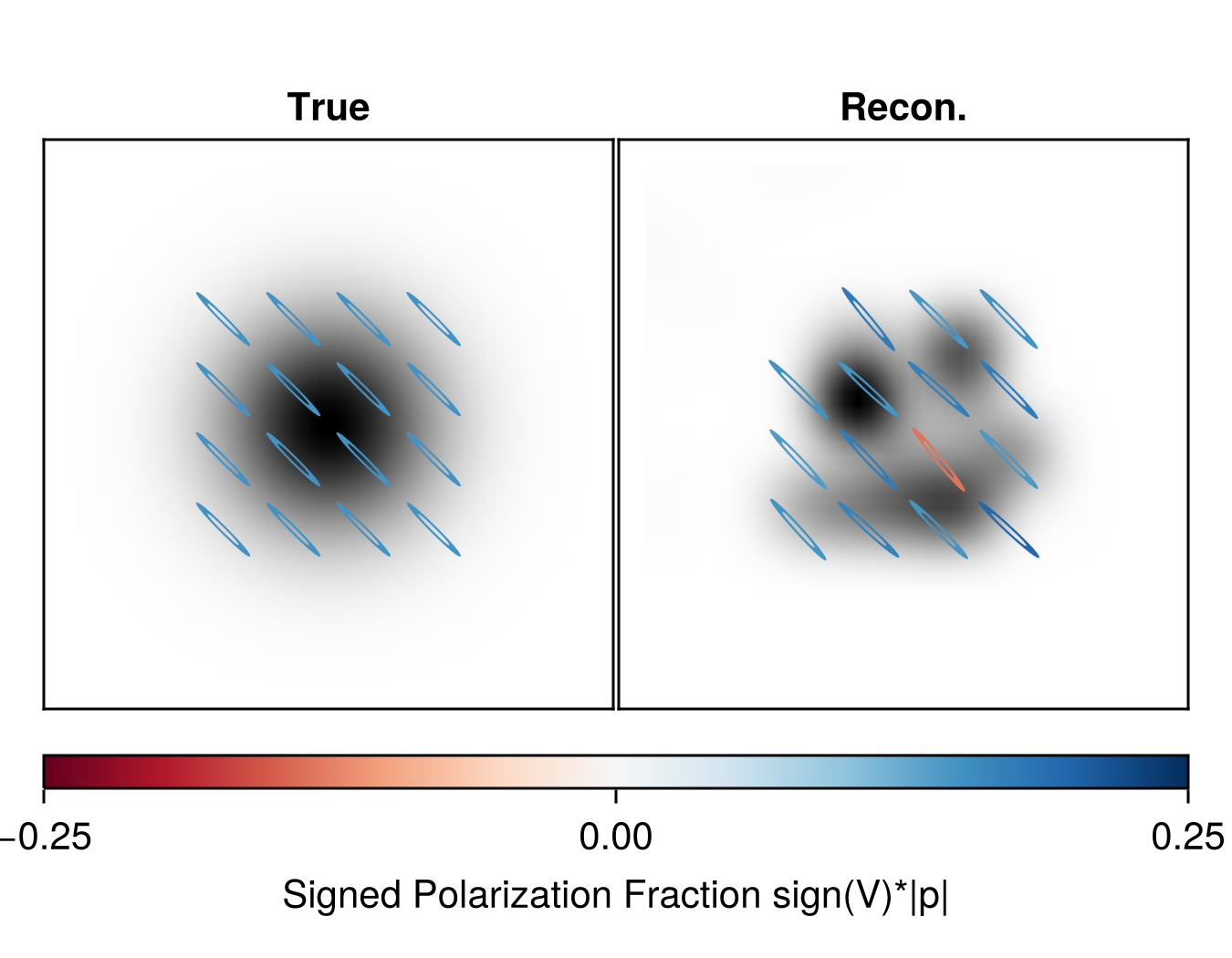

Let's compare some image statics, like the total linear polarization fraction

julia

ftrue = flux(imgtruesub);
@info "Linear polarization true image: $(abs(linearpol(ftrue))/ftrue.I)"
frecon = flux(img);
@info "Linear polarization recon image: $(abs(linearpol(frecon))/frecon.I)"

[ Info: Linear polarization true image: 0.14999999999999963
[ Info: Linear polarization recon image: 0.15137939017744853

And the Circular polarization fraction

julia

@info "Circular polarization true image: $(ftrue.V/ftrue.I)"
@info "Circular polarization recon image: $(frecon.V/frecon.I)"

[ Info: Circular polarization true image: 0.014999999999999986
[ Info: Circular polarization recon image: 0.03506935324869133

Because we also fit the instrument model, we can inspect their parameters. To do this, Comrade provides a caltable function that converts the flattened gain parameters to a tabular format based on the time and its segmentation.

julia

dR = caltable(complex.(xopt.instrument.dRx, xopt.instrument.dRy))

───────────────────────────────────────────────────┬────────────────────────────
                                              time │                    AA     ⋯
───────────────────────────────────────────────────┼────────────────────────────
 IntegrationTime{Float64}(51544, 11.8333, 23.6667) │ 0.0101847-0.0200278im  -0 ⋯
───────────────────────────────────────────────────┴────────────────────────────
                                                               6 columns omitted

We can compare this to the ground truth d-terms

time	AA	AP	AZ	JC	LM	PV	SM
0.0	0.01-0.02im	-0.08+0.07im	0.09-0.10im	-0.04+0.05im	0.03-0.02im	-0.01+0.02im	0.08-0.07im

And same for the left-handed dterms

julia

dL = caltable(complex.(xopt.instrument.dLx, xopt.instrument.dLy))

───────────────────────────────────────────────────┬────────────────────────────
                                              time │                    AA     ⋯
───────────────────────────────────────────────────┼────────────────────────────
 IntegrationTime{Float64}(51544, 11.8333, 23.6667) │ 0.0292899-0.0392239im  -0 ⋯
───────────────────────────────────────────────────┴────────────────────────────
                                                               6 columns omitted

time	AA	AP	AZ	JC	LM	PV	SM
0.0	0.03-0.04im	-0.06+0.05im	0.09-0.08im	-0.06+0.07im	0.01-0.00im	-0.03+0.04im	0.06-0.05im

Looking at the gain phase ratio

julia

gphase_ratio = caltable(xopt.instrument.gprat)

───────────────────────────────────────────────────┬────────────────────────────
                                              time │      AA           AP      ⋯
───────────────────────────────────────────────────┼────────────────────────────
      IntegrationTime{Float64}(51544, 0.0, 0.0002) │ missing      missing    m ⋯
 IntegrationTime{Float64}(51544, 0.333333, 0.0002) │ missing      missing    m ⋯
 IntegrationTime{Float64}(51544, 0.666667, 0.0002) │ missing      missing    m ⋯
      IntegrationTime{Float64}(51544, 1.0, 0.0002) │ missing      missing    m ⋯
  IntegrationTime{Float64}(51544, 1.33333, 0.0002) │ missing      missing    m ⋯
  IntegrationTime{Float64}(51544, 1.66667, 0.0002) │ missing      missing    m ⋯
  IntegrationTime{Float64}(51544, 9.66667, 0.0002) │     0.0     0.217334    m ⋯
     IntegrationTime{Float64}(51544, 10.0, 0.0002) │     0.0    0.0010218    m ⋯
  IntegrationTime{Float64}(51544, 10.3333, 0.0002) │     0.0   -0.0776836    m ⋯
  IntegrationTime{Float64}(51544, 10.6667, 0.0002) │     0.0    0.0412087    m ⋯
     IntegrationTime{Float64}(51544, 11.0, 0.0002) │     0.0    -0.121324    m ⋯
  IntegrationTime{Float64}(51544, 11.3333, 0.0002) │     0.0    0.0600191    m ⋯
  IntegrationTime{Float64}(51544, 11.6667, 0.0002) │     0.0   -0.0913795    m ⋯
     IntegrationTime{Float64}(51544, 12.0, 0.0002) │     0.0      0.03598    m ⋯
  IntegrationTime{Float64}(51544, 12.3333, 0.0002) │     0.0   -0.0163897    m ⋯
  IntegrationTime{Float64}(51544, 12.6667, 0.0002) │     0.0    0.0631087    m ⋯
                         ⋮                         │    ⋮          ⋮           ⋱
───────────────────────────────────────────────────┴────────────────────────────
                                                   5 columns and 33 rows omitted

we see that they are all very small. Which should be the case since this data doesn't have gain corruptions! Similarly our gain ratio amplitudes are also very close to unity as expected.

julia

gamp_ratio   = caltable(exp.(xopt.instrument.lgrat))

───────────────────────────────────────────────────┬────────────────────────────
                                              time │      AA       AP       AZ ⋯
───────────────────────────────────────────────────┼────────────────────────────
      IntegrationTime{Float64}(51544, 0.0, 0.0002) │ missing  missing  missing ⋯
 IntegrationTime{Float64}(51544, 0.333333, 0.0002) │ missing  missing  missing ⋯
 IntegrationTime{Float64}(51544, 0.666667, 0.0002) │ missing  missing  missing ⋯
      IntegrationTime{Float64}(51544, 1.0, 0.0002) │ missing  missing  missing ⋯
  IntegrationTime{Float64}(51544, 1.33333, 0.0002) │ missing  missing  missing ⋯
  IntegrationTime{Float64}(51544, 1.66667, 0.0002) │ missing  missing  missing ⋯
  IntegrationTime{Float64}(51544, 9.66667, 0.0002) │ 1.01624  1.04851  missing ⋯
     IntegrationTime{Float64}(51544, 10.0, 0.0002) │ 1.01744  1.02814  missing ⋯
  IntegrationTime{Float64}(51544, 10.3333, 0.0002) │ 1.02112  1.02877  missing ⋯
  IntegrationTime{Float64}(51544, 10.6667, 0.0002) │ 1.00789  1.03516  missing ⋯
     IntegrationTime{Float64}(51544, 11.0, 0.0002) │ 1.02006  1.01096  missing ⋯
  IntegrationTime{Float64}(51544, 11.3333, 0.0002) │ 1.01471  1.04777  missing ⋯
  IntegrationTime{Float64}(51544, 11.6667, 0.0002) │ 1.01986  1.00459  missing ⋯
     IntegrationTime{Float64}(51544, 12.0, 0.0002) │ 1.01944  1.02907  missing ⋯
  IntegrationTime{Float64}(51544, 12.3333, 0.0002) │ 1.02251  1.00863  missing ⋯
  IntegrationTime{Float64}(51544, 12.6667, 0.0002) │ 1.01817  1.00142  missing ⋯
                         ⋮                         │    ⋮        ⋮        ⋮    ⋱
───────────────────────────────────────────────────┴────────────────────────────
                                                   4 columns and 33 rows omitted

Plotting the gain phases, we see some offsets from zero. This is because the prior on the gain product phases is very broad, so we can't phase center the image. For realistic data this is always the case since the atmosphere effectively scrambles the phases.

julia

gphaseR = caltable(xopt.instrument.gpR)
p = Plots.plot(gphaseR, layout=(3,3), size=(650,500));
Plots.plot!(p, gphase_ratio, layout=(3,3), size=(650,500));
p |> DisplayAs.PNG |> DisplayAs.Text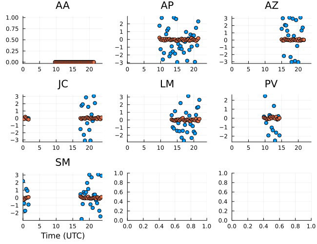

Finally, the product gain amplitudes are all very close to unity as well, as expected since gain corruptions have not been added to the data.

julia

gampr = caltable(exp.(xopt.instrument.lgR))
p = Plots.plot(gampr, layout=(3,3), size=(650,500))
Plots.plot!(p, gamp_ratio, layout=(3,3), size=(650,500))
p |> DisplayAs.PNG |> DisplayAs.Text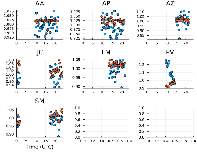

This page was generated using Literate.jl.

Hamaker J.P, Bregman J.D., Sault R.J. (1996) [https://articles.adsabs.harvard.edu/pdf/1996A%26AS..117..137H] ↩︎
Pesce D. (2021) [https://ui.adsabs.harvard.edu/abs/2021AJ....161..178P/abstract] ↩︎

Polarized Image and Instrumental Modeling ​

Introduction to Polarized Imaging ​

Load the Data ​

Load the Data ​

Reconstructing the Image and Instrument Effects ​

Polarized Image and Instrumental Modeling

Introduction to Polarized Imaging

Load the Data

Load the Data

Reconstructing the Image and Instrument Effects