Hybrid Imaging of a Black Hole
In this tutorial, we will use hybrid imaging to analyze the 2017 EHT data. By hybrid imaging, we mean decomposing the model into simple geometric models, e.g., rings and such, plus a rasterized image model to soak up the additional structure. This approach was first developed in BB20 and applied to EHT 2017 data. We will use a similar model in this tutorial.
Introduction to Hybrid modeling and imaging
The benefit of using a hybrid-based modeling approach is the effective compression of information/parameters when fitting the data. Hybrid modeling requires the user to incorporate specific knowledge of how you expect the source to look like. For instance for M87, we expect the image to be dominated by a ring-like structure. Therefore, instead of using a high-dimensional raster to recover the ring, we can use a ring model plus a raster to soak up the additional degrees of freedom. This is the approach we will take in this tutorial to analyze the April 6 2017 EHT data of M87.
Loading the Data
To get started we will load Comrade
using ComradeLoad the Data
using Pyehtim CondaPkg Found dependencies: /home/runner/.julia/packages/DimensionalData/bwTLK/CondaPkg.toml
CondaPkg Found dependencies: /home/runner/.julia/packages/PythonCall/WMWY0/CondaPkg.toml
CondaPkg Found dependencies: /home/runner/.julia/packages/Pyehtim/Fm109/CondaPkg.toml
CondaPkg Resolving changes
+ ehtim (pip)
+ libstdcxx-ng
+ numpy
+ numpy (pip)
+ openssl
+ pandas
+ python
+ setuptools (pip)
+ uv
+ xarray
CondaPkg Creating environment
│ /home/runner/.julia/artifacts/7973f2c7725e2d0eef7a95159454c4145f0945a2/bin/micromamba
│ -r /home/runner/.julia/scratchspaces/0b3b1443-0f03-428d-bdfb-f27f9c1191ea/root
│ create
│ -y
│ -p /home/runner/work/Comrade.jl/Comrade.jl/examples/advanced/HybridImaging/.CondaPkg/env
│ --override-channels
│ --no-channel-priority
│ libstdcxx-ng[version='>=3.4,<13.0']
│ numpy[version='*']
│ numpy[version='>=1.24, <2.0']
│ openssl[version='>=3, <3.1']
│ pandas[version='<2']
│ python[version='>=3.8,<4',channel='conda-forge',build='*cpython*']
│ python[version='>=3.6,<=3.10']
│ uv[version='>=0.4']
│ xarray[version='*']
└ -c conda-forge
Transaction
Prefix: /home/runner/work/Comrade.jl/Comrade.jl/examples/advanced/HybridImaging/.CondaPkg/env
Updating specs:
- libstdcxx-ng[version='>=3.4,<13.0']
- numpy=*
- numpy[version='>=1.24, <2.0']
- openssl[version='>=3, <3.1']
- pandas[version='<2']
- conda-forge::python[version='>=3.8,<4',build=*cpython*]
- python[version='>=3.6,<=3.10']
- uv[version='>=0.4']
- xarray=*
Package Version Build Channel Size
─────────────────────────────────────────────────────────────────────────────────
Install:
─────────────────────────────────────────────────────────────────────────────────
+ libstdcxx-ng 12.3.0 hc0a3c3a_7 conda-forge Cached
+ _libgcc_mutex 0.1 conda_forge conda-forge Cached
+ python_abi 3.10 5_cp310 conda-forge Cached
+ ca-certificates 2024.12.14 hbcca054_0 conda-forge Cached
+ ld_impl_linux-64 2.43 h712a8e2_2 conda-forge Cached
+ libgomp 14.2.0 h77fa898_1 conda-forge Cached
+ _openmp_mutex 4.5 2_gnu conda-forge Cached
+ libgcc 14.2.0 h77fa898_1 conda-forge Cached
+ liblzma 5.6.3 hb9d3cd8_1 conda-forge Cached
+ ncurses 6.5 h2d0b736_3 conda-forge Cached
+ libzlib 1.3.1 hb9d3cd8_2 conda-forge Cached
+ libgfortran5 14.2.0 hd5240d6_1 conda-forge Cached
+ libstdcxx 14.2.0 hc0a3c3a_1 conda-forge Cached
+ libgcc-ng 14.2.0 h69a702a_1 conda-forge Cached
+ xz-tools 5.6.3 hb9d3cd8_1 conda-forge Cached
+ xz-gpl-tools 5.6.3 hbcc6ac9_1 conda-forge Cached
+ liblzma-devel 5.6.3 hb9d3cd8_1 conda-forge Cached
+ libsqlite 3.48.0 hee588c1_1 conda-forge Cached
+ libgfortran 14.2.0 h69a702a_1 conda-forge Cached
+ uv 0.5.25 h0f3a69f_0 conda-forge Cached
+ tk 8.6.13 noxft_h4845f30_101 conda-forge Cached
+ readline 8.2 h8228510_1 conda-forge Cached
+ libuuid 2.38.1 h0b41bf4_0 conda-forge Cached
+ libnsl 2.0.1 hd590300_0 conda-forge Cached
+ libffi 3.4.2 h7f98852_5 conda-forge Cached
+ bzip2 1.0.8 h4bc722e_7 conda-forge Cached
+ openssl 3.0.14 h4ab18f5_0 conda-forge Cached
+ xz 5.6.3 hbcc6ac9_1 conda-forge Cached
+ libopenblas 0.3.28 pthreads_h94d23a6_1 conda-forge Cached
+ sqlite 3.48.0 h9eae976_1 conda-forge Cached
+ libblas 3.9.0 28_h59b9bed_openblas conda-forge Cached
+ libcblas 3.9.0 28_he106b2a_openblas conda-forge Cached
+ liblapack 3.9.0 28_h7ac8fdf_openblas conda-forge Cached
+ tzdata 2025a h78e105d_0 conda-forge Cached
+ python 3.10.0 h543edf9_3_cpython conda-forge Cached
+ wheel 0.45.1 pyhd8ed1ab_1 conda-forge Cached
+ setuptools 75.8.0 pyhff2d567_0 conda-forge Cached
+ pip 25.0 pyh8b19718_0 conda-forge Cached
+ six 1.17.0 pyhd8ed1ab_0 conda-forge Cached
+ pytz 2024.2 pyhd8ed1ab_1 conda-forge Cached
+ packaging 24.2 pyhd8ed1ab_2 conda-forge Cached
+ python-dateutil 2.9.0.post0 pyhff2d567_1 conda-forge Cached
+ numpy 1.26.4 py310hb13e2d6_0 conda-forge Cached
+ pandas 1.5.3 py310h9b08913_1 conda-forge Cached
+ xarray 2024.3.0 pyhd8ed1ab_0 conda-forge Cached
Summary:
Install: 45 packages
Total download: 0 B
─────────────────────────────────────────────────────────────────────────────────
Transaction starting
Linking libstdcxx-ng-12.3.0-hc0a3c3a_7
Linking _libgcc_mutex-0.1-conda_forge
Linking python_abi-3.10-5_cp310
Linking ca-certificates-2024.12.14-hbcca054_0
Linking ld_impl_linux-64-2.43-h712a8e2_2
Linking libgomp-14.2.0-h77fa898_1
Linking _openmp_mutex-4.5-2_gnu
Linking libgcc-14.2.0-h77fa898_1
Linking liblzma-5.6.3-hb9d3cd8_1
Linking ncurses-6.5-h2d0b736_3
Linking libzlib-1.3.1-hb9d3cd8_2
Linking libgfortran5-14.2.0-hd5240d6_1
Linking libstdcxx-14.2.0-hc0a3c3a_1
warning libmamba [libstdcxx-14.2.0-hc0a3c3a_1] The following files were already present in the environment:
- lib/libstdc++.so
- lib/libstdc++.so.6
- share/licenses/libstdc++/RUNTIME.LIBRARY.EXCEPTION
Linking libgcc-ng-14.2.0-h69a702a_1
Linking xz-tools-5.6.3-hb9d3cd8_1
Linking xz-gpl-tools-5.6.3-hbcc6ac9_1
Linking liblzma-devel-5.6.3-hb9d3cd8_1
Linking libsqlite-3.48.0-hee588c1_1
Linking libgfortran-14.2.0-h69a702a_1
Linking uv-0.5.25-h0f3a69f_0
Linking tk-8.6.13-noxft_h4845f30_101
Linking readline-8.2-h8228510_1
Linking libuuid-2.38.1-h0b41bf4_0
Linking libnsl-2.0.1-hd590300_0
Linking libffi-3.4.2-h7f98852_5
Linking bzip2-1.0.8-h4bc722e_7
Linking openssl-3.0.14-h4ab18f5_0
Linking xz-5.6.3-hbcc6ac9_1
Linking libopenblas-0.3.28-pthreads_h94d23a6_1
Linking sqlite-3.48.0-h9eae976_1
Linking libblas-3.9.0-28_h59b9bed_openblas
Linking libcblas-3.9.0-28_he106b2a_openblas
Linking liblapack-3.9.0-28_h7ac8fdf_openblas
Linking tzdata-2025a-h78e105d_0
Linking python-3.10.0-h543edf9_3_cpython
Linking wheel-0.45.1-pyhd8ed1ab_1
Linking setuptools-75.8.0-pyhff2d567_0
Linking pip-25.0-pyh8b19718_0
Linking six-1.17.0-pyhd8ed1ab_0
Linking pytz-2024.2-pyhd8ed1ab_1
Linking packaging-24.2-pyhd8ed1ab_2
Linking python-dateutil-2.9.0.post0-pyhff2d567_1
Linking numpy-1.26.4-py310hb13e2d6_0
Linking pandas-1.5.3-py310h9b08913_1
Linking xarray-2024.3.0-pyhd8ed1ab_0
Transaction finished
To activate this environment, use:
micromamba activate /home/runner/work/Comrade.jl/Comrade.jl/examples/advanced/HybridImaging/.CondaPkg/env
Or to execute a single command in this environment, use:
micromamba run -p /home/runner/work/Comrade.jl/Comrade.jl/examples/advanced/HybridImaging/.CondaPkg/env mycommand
CondaPkg Installing Pip packages
│ /home/runner/work/Comrade.jl/Comrade.jl/examples/advanced/HybridImaging/.CondaPkg/env/bin/uv
│ pip
│ install
│ ehtim >=1.2.10, <2.0
│ numpy >=1.24, <2.0
└ setuptools
Using Python 3.10.0 environment at: /home/runner/work/Comrade.jl/Comrade.jl/examples/advanced/HybridImaging/.CondaPkg/env
Resolved 35 packages in 12ms
Installed 29 packages in 50ms
+ astropy==6.1.7
+ astropy-iers-data==0.2025.1.27.0.32.44
+ certifi==2024.12.14
+ charset-normalizer==3.4.1
+ contourpy==1.3.1
+ cycler==0.12.1
+ ehtim==1.2.10
+ fonttools==4.55.8
+ future==1.0.0
+ h5py==3.12.1
+ hdrhistogram==0.10.3
+ idna==3.10
+ jplephem==2.22
+ kiwisolver==1.4.8
+ matplotlib==3.10.0
+ networkx==3.4.2
+ pandas-appender==0.9.9
+ paramsurvey==0.4.21
+ pbr==6.1.0
+ pillow==11.1.0
+ psutil==6.1.1
+ pyerfa==2.0.1.5
+ pyparsing==3.2.1
+ pyyaml==6.0.2
+ requests==2.32.3
+ scipy==1.15.1
+ sgp4==2.23
+ skyfield==1.49
+ urllib3==2.3.0For reproducibility we use a stable random number genreator
using StableRNGs
rng = StableRNG(11)StableRNGs.LehmerRNG(state=0x00000000000000000000000000000017)To download the data visit https://doi.org/10.25739/g85n-f134 To load the eht-imaging obsdata object we do:
obs = ehtim.obsdata.load_uvfits(joinpath(__DIR, "..", "..", "Data", "SR1_M87_2017_096_lo_hops_netcal_StokesI.uvfits"))Python: <ehtim.obsdata.Obsdata object at 0x7f112b210c10>Now we do some minor preprocessing:
- Scan average the data since the data have been preprocessed so that the gain phases coherent.
obs = scan_average(obs).add_fractional_noise(0.02)Python: <ehtim.obsdata.Obsdata object at 0x7f112cd35240>For this tutorial we will once again fit complex visibilities since they provide the most information once the telescope/instrument model are taken into account.
dvis = extract_table(obs, Visibilities())EHTObservationTable{Comrade.EHTVisibilityDatum{:I}}
source: M87
mjd: 57849
bandwidth: 1.856e9
sites: [:AA, :AP, :AZ, :JC, :LM, :PV, :SM]
nsamples: 274Building the Model/Posterior
Now we build our intensity/visibility model. That is, the model that takes in a named tuple of parameters and perhaps some metadata required to construct the model. For our model, we will use a raster or ContinuousImage model, an m-ring model, and a large asymmetric Gaussian component to model the unresolved short-baseline flux.
function sky(θ, metadata)
    (;c, σimg, f, r, σ, ma, mp, fg) = θ
    (;ftot, grid) = metadata
    # Form the image model
    # First transform to simplex space first applying the non-centered transform
    rast = (ftot*f*(1-fg)).*to_simplex(CenteredLR(), σimg.*c)
    mimg = ContinuousImage(rast, grid, BSplinePulse{3}())
    # Form the ring model
    α = ma.*cos.(mp)
    β = ma.*sin.(mp)
    ring = smoothed(modify(MRing(α, β), Stretch(r), Renormalize((ftot*(1-f)*(1-fg)))), σ)
    gauss = modify(Gaussian(), Stretch(μas2rad(250.0)), Renormalize(ftot*f*fg))
    # We group the geometric models together for improved efficiency. This will be
    # automated in future versions.
    return mimg + (ring + gauss)
end
sky (generic function with 1 method)Unlike other imaging examples (e.g., Imaging a Black Hole using only Closure Quantities) we also need to include a model for the instrument, i.e., gains as well. The gains will be broken into two components
Gain amplitudes which are typically known to 10-20%, except for LMT, which has amplitudes closer to 50-100%.
Gain phases which are more difficult to constrain and can shift rapidly.
using VLBIImagePriors
using Distributions
fgain(x) = exp(x.lg + 1im*x.gp)
G = SingleStokesGain(fgain)

intpr = (
    lg= ArrayPrior(IIDSitePrior(ScanSeg(), Normal(0.0, 0.2)); LM = IIDSitePrior(ScanSeg(), Normal(0.0, 1.0))),
    gp= ArrayPrior(IIDSitePrior(ScanSeg(), DiagonalVonMises(0.0, inv(π^2))); refant=SEFDReference(0.0))
        )
intmodel = InstrumentModel(G, intpr)
InstrumentModel
with Jones: SingleStokesGain
with reference basis: PolarizedTypes.CirBasis()Before we move on, let's go into the model function a bit. This function takes two arguments θ and metadata. The θ argument is a named tuple of parameters that are fit to the data. The metadata argument is all the ancillary information we need to construct the model. For our hybrid model, we will need two variables for the metadata, a grid that specifies the locations of the image pixels and a cache that defines the algorithm used to calculate the visibilities given the image model. This is required since ContinuousImage is most easily computed using number Fourier transforms like the NFFT or FFT. To combine the models, we use Comrade's overloaded + operators, which will combine the images such that their intensities and visibilities are added pointwise.
Now let's define our metadata. First we will define the cache for the image. This is required to compute the numerical Fourier transform.
fovxy  = μas2rad(200.0)
npix   = 32
g      = imagepixels(fovxy, fovxy, npix, npix)
RectiGrid(
executor: ComradeBase.Serial()
Dimensions:
(↓ X Sampled{Float64} LinRange{Float64}(-4.69663253574863e-10, 4.69663253574863e-10, 32) ForwardOrdered Regular Points,
→ Y Sampled{Float64} LinRange{Float64}(-4.69663253574863e-10, 4.69663253574863e-10, 32) ForwardOrdered Regular Points)
)Part of hybrid imaging is to force a scale separation between the different model components to make them identifiable. To enforce this we will set the raster component to have a correlation length of 5 times the beam size.
beam = beamsize(dvis)
rat = (beam/(step(g.X)))
cprior = GaussMarkovRandomField(5*rat, size(g))
VLBIImagePriors.GaussMarkovRandomField(
Graph: MarkovRandomFieldGraph{1}(
dims: (32, 32)
)
Correlation Parameter: 19.9737623915157
)For the other parameters we use a uniform priors for the ring fractional flux f ring radius r, ring width σ, and the flux fraction of the Gaussian component fg and the amplitude for the ring brightness modes. For the angular variables ξτ and ξ we use the von Mises prior with concentration parameter inv(π^2) which is essentially a uniform prior on the circle. Finally for the standard deviation of the MRF we use a half-normal distribution. This is to ensure that the MRF has small differences from the mean image.
skyprior = (
          c  = cprior,
          σimg = truncated(Normal(0.0, 0.1); lower=0.01),
          f  = Uniform(0.0, 1.0),
          r  = Uniform(μas2rad(10.0), μas2rad(30.0)),
          σ  = Uniform(μas2rad(0.1), μas2rad(10.0)),
          ma = ntuple(_->Uniform(0.0, 0.5), 2),
          mp = ntuple(_->DiagonalVonMises(0.0, inv(π^2)), 2),
          fg = Uniform(0.0, 1.0),
        )
(c = VLBIImagePriors.GaussMarkovRandomField(
Graph: MarkovRandomFieldGraph{1}(
dims: (32, 32)
)
Correlation Parameter: 19.9737623915157
), σimg = Truncated(Distributions.Normal{Float64}(μ=0.0, σ=0.1); lower=0.01), f = Distributions.Uniform{Float64}(a=0.0, b=1.0), r = Distributions.Uniform{Float64}(a=4.84813681109536e-11, b=1.454441043328608e-10), σ = Distributions.Uniform{Float64}(a=4.848136811095359e-13, b=4.84813681109536e-11), ma = (Distributions.Uniform{Float64}(a=0.0, b=0.5), Distributions.Uniform{Float64}(a=0.0, b=0.5)), mp = (VLBIImagePriors.DiagonalVonMises{Float64, Float64, Float64}(μ=0.0, κ=0.10132118364233778, lnorm=-1.739120733481688), VLBIImagePriors.DiagonalVonMises{Float64, Float64, Float64}(μ=0.0, κ=0.10132118364233778, lnorm=-1.739120733481688)), fg = Distributions.Uniform{Float64}(a=0.0, b=1.0))Now we form the metadata
skymetadata = (;ftot=1.1, grid = g)
skym = SkyModel(sky, skyprior, g; metadata=skymetadata)
SkyModel
with map: sky
on grid: ComradeBase.RectiGridThis is everything we need to specify our posterior distribution, which our is the main object of interest in image reconstructions when using Bayesian inference.
using Enzyme
post = VLBIPosterior(skym, intmodel, dvis; admode=set_runtime_activity(Enzyme.Reverse))
VLBIPosterior
ObservedSkyModel
with map: sky
on grid: VLBISkyModels.FourierDualDomainObservedInstrumentModel
with Jones: SingleStokesGain
with reference basis: PolarizedTypes.CirBasis()Data Products: Comrade.EHTVisibilityDatumWe can sample from the prior to see what the model looks like
import CairoMakie as CM
xrand = prior_sample(rng, post)
gpl = imagepixels(μas2rad(200.0), μas2rad(200.0), 128, 128)
fig = imageviz(intensitymap(skymodel(post, xrand), gpl));
Reconstructing the Image
To find the image we will demonstrate two methods:
Optimization to find the MAP (fast but often a poor estimator)
Sampling to find the posterior (slow but provides a substantially better estimator)
For optimization we will use the Optimization.jl package and the LBFGS optimizer. To use this we use the comrade_opt function
using Optimization
using OptimizationOptimJL
xopt, sol = comrade_opt(post, LBFGS();
                        initial_params=xrand, maxiters=2000, g_tol=1e0);
┌ Warning: TODO forward zero-set of arraycopy used memset rather than runtime type
│ Caused by:
│ Stacktrace:
│ [1] copy
│ @ ./array.jl:411
│ [2] map
│ @ ./tuple.jl:293
│ [3] map
│ @ ./tuple.jl:294
│ [4] map
│ @ ./namedtuple.jl:265
│ [5] copy
│ @ ~/.julia/packages/StructArrays/KLKnN/src/structarray.jl:467
└ @ Enzyme.Compiler ~/.julia/packages/GPUCompiler/Nxf8r/src/utils.jl:59
┌ Warning: TODO forward zero-set of arraycopy used memset rather than runtime type
│ Caused by:
│ Stacktrace:
│ [1] copy
│ @ ./array.jl:411
│ [2] map
│ @ ./tuple.jl:294
│ [3] map
│ @ ./namedtuple.jl:265
│ [4] copy
│ @ ~/.julia/packages/StructArrays/KLKnN/src/structarray.jl:467
└ @ Enzyme.Compiler ~/.julia/packages/GPUCompiler/Nxf8r/src/utils.jl:59
┌ Warning: TODO forward zero-set of arraycopy used memset rather than runtime type
│ Caused by:
│ Stacktrace:
│ [1] copy
│ @ ./array.jl:411
│ [2] map
│ @ ./tuple.jl:293
│ [3] map
│ @ ./tuple.jl:294
│ [4] map
│ @ ./namedtuple.jl:265
│ [5] copy
│ @ ~/.julia/packages/StructArrays/KLKnN/src/structarray.jl:467
└ @ Enzyme.Compiler ~/.julia/packages/GPUCompiler/Nxf8r/src/utils.jl:59
┌ Warning: TODO forward zero-set of arraycopy used memset rather than runtime type
│ Caused by:
│ Stacktrace:
│ [1] copy
│ @ ./array.jl:411
│ [2] map
│ @ ./tuple.jl:294
│ [3] map
│ @ ./namedtuple.jl:265
│ [4] copy
│ @ ~/.julia/packages/StructArrays/KLKnN/src/structarray.jl:467
└ @ Enzyme.Compiler ~/.julia/packages/GPUCompiler/Nxf8r/src/utils.jl:59First we will evaluate our fit by plotting the residuals
using Plots
fig = residual(post, xopt);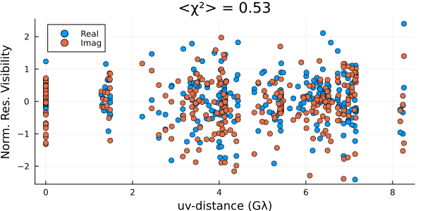
These residuals suggest that we are substantially overfitting the data. This is a common side effect of MAP imaging. As a result if we plot the image we see that there is substantial high-frequency structure in the image that isn't supported by the data.
fig = imageviz(intensitymap(skymodel(post, xopt), gpl), figure=(;resolution=(500, 400),));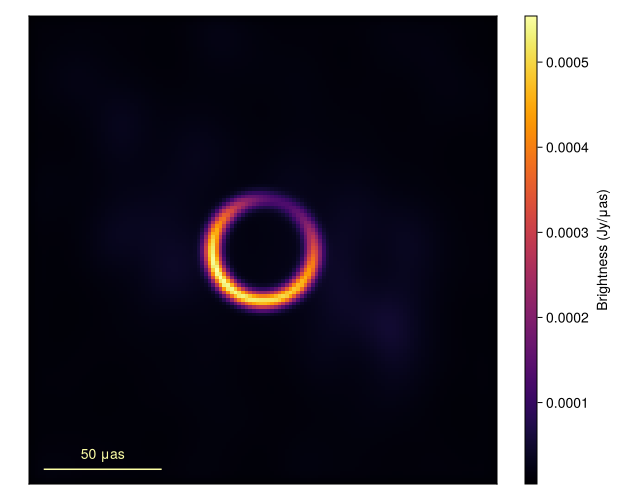
To improve our results we will now move to Posterior sampling. This is the main method we recommend for all inference problems in Comrade. While it is slower the results are often substantially better. To sample we will use the AdvancedHMC package.
using AdvancedHMC
chain = sample(rng, post, NUTS(0.8), 700; n_adapts=500, progress=false, initial_params=xopt);
[ Info: Found initial step size 0.003125We then remove the adaptation/warmup phase from our chain
chain = chain[501:end]PosteriorSamples
Samples size: (200,)
sampler used: AHMC
Mean
┌──────────────────────────────────────────────────────────────────────────────────────────────────────────────────────────────────────────────────────────────────────────────────────────────────────────────────────────────────────────────────────────────────────────────────────────────────────────────────────────────┬───────────────────────────────────────────────────────────────────────────────────────────────────────────────────────────────────────────────────────────────────────────────────────────────────────────────────────────────────────────────────────────────────────────────────────────────────────────────────────────────────────────────────────────────────────────────────────────────────────────────────────────────────────────┐
│ sky │ instrument │
│ @NamedTuple{c::Matrix{Float64}, σimg::Float64, f::Float64, r::Float64, σ::Float64, ma::Tuple{Float64, Float64}, mp::Tuple{Float64, Float64}, fg::Float64} │ @NamedTuple{lg::Comrade.SiteArray{Float64, 1, Vector{Float64}, Vector{Comrade.IntegrationTime{Int64, Float64}}, Vector{Comrade.FrequencyChannel{Float64, Int64}}, Vector{Symbol}}, gp::Comrade.SiteArray{Float64, 1, Vector{Float64}, Vector{Comrade.IntegrationTime{Int64, Float64}}, Vector{Comrade.FrequencyChannel{Float64, Int64}}, Vector{Symbol}}} │
├──────────────────────────────────────────────────────────────────────────────────────────────────────────────────────────────────────────────────────────────────────────────────────────────────────────────────────────────────────────────────────────────────────────────────────────────────────────────────────────────┼───────────────────────────────────────────────────────────────────────────────────────────────────────────────────────────────────────────────────────────────────────────────────────────────────────────────────────────────────────────────────────────────────────────────────────────────────────────────────────────────────────────────────────────────────────────────────────────────────────────────────────────────────────────┤
│ (c = [-0.109304 -0.207339 … -0.369345 -0.240965; -0.173374 -0.277786 … -0.382463 -0.237717; … ; 0.153553 0.0543502 … -0.148655 -0.120507; 0.0886018 0.0664537 … -0.108598 -0.0595397], σimg = 0.608641, f = 0.683232, r = 1.04806e-10, σ = 1.20285e-11, ma = (0.278002, 0.0615678), mp = (2.67454, 2.18906), fg = 0.0912916) │ (lg = [0.0367071, 0.0163548, 0.029724, 0.0374606, -0.206013, 0.115218, 0.0207811, 0.0427358, -0.0102788, 0.0786809 … 0.0268941, 0.0276426, -0.673404, 0.0276532, 0.0210533, 0.0434551, -0.0338541, 0.0353314, -0.713782, 0.0241352], gp = [0.0, 0.0877529, 0.0, -2.19108, 1.418, -0.0690189, 0.0, -2.2402, 1.47446, -0.272356 … -1.80879, -0.0111991, -2.74538, -0.0226104, 0.0, -1.82829, -1.91676, 0.0120532, -2.88206, -0.695572]) │
└──────────────────────────────────────────────────────────────────────────────────────────────────────────────────────────────────────────────────────────────────────────────────────────────────────────────────────────────────────────────────────────────────────────────────────────────────────────────────────────────┴───────────────────────────────────────────────────────────────────────────────────────────────────────────────────────────────────────────────────────────────────────────────────────────────────────────────────────────────────────────────────────────────────────────────────────────────────────────────────────────────────────────────────────────────────────────────────────────────────────────────────────────────────────────┘
Std. Dev.
┌────────────────────────────────────────────────────────────────────────────────────────────────────────────────────────────────────────────────────────────────────────────────────────────────────────────────────────────────────────────────────────────────────────────────────────────────────────────┬────────────────────────────────────────────────────────────────────────────────────────────────────────────────────────────────────────────────────────────────────────────────────────────────────────────────────────────────────────────────────────────────────────────────────────────────────────────────────────────────────────────────────────────────────────────────────────────────────────────────────────────────────────────┐
│ sky │ instrument │
│ @NamedTuple{c::Matrix{Float64}, σimg::Float64, f::Float64, r::Float64, σ::Float64, ma::Tuple{Float64, Float64}, mp::Tuple{Float64, Float64}, fg::Float64} │ @NamedTuple{lg::Comrade.SiteArray{Float64, 1, Vector{Float64}, Vector{Comrade.IntegrationTime{Int64, Float64}}, Vector{Comrade.FrequencyChannel{Float64, Int64}}, Vector{Symbol}}, gp::Comrade.SiteArray{Float64, 1, Vector{Float64}, Vector{Comrade.IntegrationTime{Int64, Float64}}, Vector{Comrade.FrequencyChannel{Float64, Int64}}, Vector{Symbol}}} │
├────────────────────────────────────────────────────────────────────────────────────────────────────────────────────────────────────────────────────────────────────────────────────────────────────────────────────────────────────────────────────────────────────────────────────────────────────────────┼────────────────────────────────────────────────────────────────────────────────────────────────────────────────────────────────────────────────────────────────────────────────────────────────────────────────────────────────────────────────────────────────────────────────────────────────────────────────────────────────────────────────────────────────────────────────────────────────────────────────────────────────────────────┤
│ (c = [0.533359 0.579351 … 0.500182 0.4856; 0.510733 0.635561 … 0.564079 0.566524; … ; 0.545685 0.605027 … 0.565071 0.569145; 0.569511 0.580688 … 0.567385 0.522293], σimg = 0.0450262, f = 0.027818, r = 1.16334e-12, σ = 5.12944e-12, ma = (0.0298236, 0.0207173), mp = (0.10111, 1.1083), fg = 0.056056) │ (lg = [0.135975, 0.142976, 0.0221066, 0.0212064, 0.0841321, 0.065811, 0.0212268, 0.0223608, 0.0727401, 0.0656533 … 0.0469926, 0.0205491, 0.0760892, 0.0204306, 0.022219, 0.0226248, 0.048861, 0.020848, 0.0809859, 0.0200805], gp = [0.0, 0.0626523, 0.0, 0.0190631, 0.0754195, 0.0613536, 0.0, 0.0184922, 0.0759814, 0.0629908 … 0.0805604, 0.0752108, 0.0802947, 3.08754, 0.0, 0.0185385, 0.0811788, 0.0732026, 0.0836364, 3.00824]) │
└────────────────────────────────────────────────────────────────────────────────────────────────────────────────────────────────────────────────────────────────────────────────────────────────────────────────────────────────────────────────────────────────────────────────────────────────────────────┴────────────────────────────────────────────────────────────────────────────────────────────────────────────────────────────────────────────────────────────────────────────────────────────────────────────────────────────────────────────────────────────────────────────────────────────────────────────────────────────────────────────────────────────────────────────────────────────────────────────────────────────────────────────┘Warning
This should be run for 4-5x more steps to properly estimate expectations of the posterior
Now lets plot the mean image and standard deviation images. To do this we first clip the first 250 MCMC steps since that is during tuning and so the posterior is not sampling from the correct sitesary distribution.
using StatsBase
msamples = skymodel.(Ref(post), chain[begin:2:end]);
The mean image is then given by
imgs = intensitymap.(msamples, Ref(gpl))
fig = imageviz(mean(imgs), colormap=:afmhot, size=(400, 300));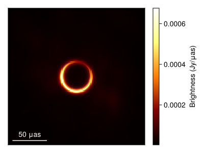
fig = imageviz(std(imgs), colormap=:batlow, size=(400, 300));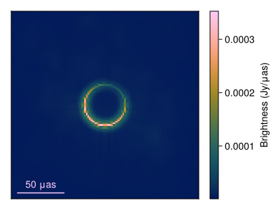
We can also split up the model into its components and analyze each separately
comp = Comrade.components.(msamples)
ring_samples = getindex.(comp, 2)
rast_samples = first.(comp)
ring_imgs = intensitymap.(ring_samples, Ref(gpl));
rast_imgs = intensitymap.(rast_samples, Ref(gpl));

ring_mean, ring_std = mean_and_std(ring_imgs);
rast_mean, rast_std = mean_and_std(rast_imgs);

fig = CM.Figure(; resolution=(400, 400));
axes = [CM.Axis(fig[i, j], xreversed=true, aspect=CM.DataAspect()) for i in 1:2, j in 1:2]
CM.image!(axes[1,1], ring_mean, colormap=:afmhot); axes[1,1].title = "Ring Mean"
CM.image!(axes[1,2], ring_std, colormap=:afmhot); axes[1,2].title = "Ring Std. Dev."
CM.image!(axes[2,1], rast_mean, colormap=:afmhot); axes[2,1].title = "Rast Mean"
CM.image!(axes[2,2], rast_std./rast_mean, colormap=:afmhot); axes[2,2].title = "Rast std/mean"
CM.hidedecorations!.(axes)
fig |> DisplayAs.PNG |> DisplayAs.Text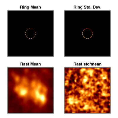
Finally, let's take a look at some of the ring parameters
figd = CM.Figure(;resolution=(650, 400));
p1 = CM.density(figd[1,1], rad2μas(chain.sky.r)*2, axis=(xlabel="Ring Diameter (μas)",))
p2 = CM.density(figd[1,2], rad2μas(chain.sky.σ)*2*sqrt(2*log(2)), axis=(xlabel="Ring FWHM (μas)",))
p3 = CM.density(figd[1,3], -rad2deg.(chain.sky.mp.:1) .+ 360.0, axis=(xlabel = "Ring PA (deg) E of N",))
p4 = CM.density(figd[2,1], 2*chain.sky.ma.:2, axis=(xlabel="Brightness asymmetry",))
p5 = CM.density(figd[2,2], 1 .- chain.sky.f, axis=(xlabel="Ring flux fraction",))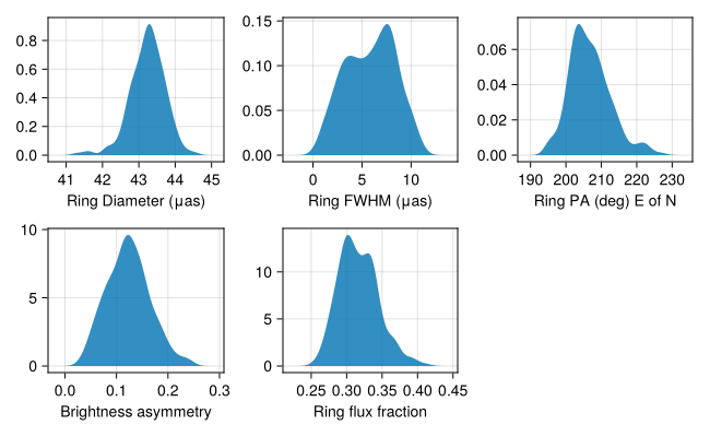
Now let's check the residuals using draws from the posterior
p = Plots.plot();
for s in sample(chain, 10)
    residual!(p, post, s, legend=false)
end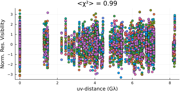
And everything looks pretty good! Now comes the hard part: interpreting the results...
This page was generated using Literate.jl.