Geometric Modeling of EHT Data
Comrade has been designed to work with the EHT and ngEHT. In this tutorial, we will show how to reproduce some of the results from EHTC VI 2019.
In EHTC VI, they considered fitting simple geometric models to the data to estimate the black hole's image size, shape, brightness profile, etc. In this tutorial, we will construct a similar model and fit it to the data in under 50 lines of code (sans comments). To start, we load Comrade and some other packages we need.
To get started we load Comrade.
using ComradeCurrently we use eht-imaging for data management, however this will soon be replaced by a pure Julia solution.
using Pyehtim CondaPkg Found dependencies: /home/runner/.julia/packages/DimensionalData/bwTLK/CondaPkg.toml
CondaPkg Found dependencies: /home/runner/.julia/packages/PythonCall/WMWY0/CondaPkg.toml
CondaPkg Found dependencies: /home/runner/.julia/packages/Pyehtim/Fm109/CondaPkg.toml
CondaPkg Resolving changes
+ ehtim (pip)
+ libstdcxx-ng
+ numpy
+ numpy (pip)
+ openssl
+ pandas
+ python
+ setuptools (pip)
+ uv
+ xarray
CondaPkg Creating environment
│ /home/runner/.julia/artifacts/7973f2c7725e2d0eef7a95159454c4145f0945a2/bin/micromamba
│ -r /home/runner/.julia/scratchspaces/0b3b1443-0f03-428d-bdfb-f27f9c1191ea/root
│ create
│ -y
│ -p /home/runner/work/Comrade.jl/Comrade.jl/examples/beginner/GeometricModeling/.CondaPkg/env
│ --override-channels
│ --no-channel-priority
│ libstdcxx-ng[version='>=3.4,<13.0']
│ numpy[version='*']
│ numpy[version='>=1.24, <2.0']
│ openssl[version='>=3, <3.1']
│ pandas[version='<2']
│ python[version='>=3.8,<4',channel='conda-forge',build='*cpython*']
│ python[version='>=3.6,<=3.10']
│ uv[version='>=0.4']
│ xarray[version='*']
└ -c conda-forge
conda-forge/linux-64 Using cache
conda-forge/noarch Using cache
Transaction
Prefix: /home/runner/work/Comrade.jl/Comrade.jl/examples/beginner/GeometricModeling/.CondaPkg/env
Updating specs:
- libstdcxx-ng[version='>=3.4,<13.0']
- numpy=*
- numpy[version='>=1.24, <2.0']
- openssl[version='>=3, <3.1']
- pandas[version='<2']
- conda-forge::python[version='>=3.8,<4',build=*cpython*]
- python[version='>=3.6,<=3.10']
- uv[version='>=0.4']
- xarray=*
Package Version Build Channel Size
─────────────────────────────────────────────────────────────────────────────────
Install:
─────────────────────────────────────────────────────────────────────────────────
+ libstdcxx-ng 12.3.0 hc0a3c3a_7 conda-forge Cached
+ _libgcc_mutex 0.1 conda_forge conda-forge Cached
+ python_abi 3.10 5_cp310 conda-forge Cached
+ ca-certificates 2024.12.14 hbcca054_0 conda-forge Cached
+ ld_impl_linux-64 2.43 h712a8e2_2 conda-forge Cached
+ libgomp 14.2.0 h77fa898_1 conda-forge Cached
+ _openmp_mutex 4.5 2_gnu conda-forge Cached
+ libgcc 14.2.0 h77fa898_1 conda-forge Cached
+ liblzma 5.6.3 hb9d3cd8_1 conda-forge Cached
+ ncurses 6.5 h2d0b736_3 conda-forge Cached
+ libzlib 1.3.1 hb9d3cd8_2 conda-forge Cached
+ libgfortran5 14.2.0 hd5240d6_1 conda-forge Cached
+ libstdcxx 14.2.0 hc0a3c3a_1 conda-forge Cached
+ libgcc-ng 14.2.0 h69a702a_1 conda-forge Cached
+ xz-tools 5.6.3 hb9d3cd8_1 conda-forge Cached
+ xz-gpl-tools 5.6.3 hbcc6ac9_1 conda-forge Cached
+ liblzma-devel 5.6.3 hb9d3cd8_1 conda-forge Cached
+ libsqlite 3.48.0 hee588c1_1 conda-forge Cached
+ libgfortran 14.2.0 h69a702a_1 conda-forge Cached
+ uv 0.5.25 h0f3a69f_0 conda-forge Cached
+ tk 8.6.13 noxft_h4845f30_101 conda-forge Cached
+ readline 8.2 h8228510_1 conda-forge Cached
+ libuuid 2.38.1 h0b41bf4_0 conda-forge Cached
+ libnsl 2.0.1 hd590300_0 conda-forge Cached
+ libffi 3.4.2 h7f98852_5 conda-forge Cached
+ bzip2 1.0.8 h4bc722e_7 conda-forge Cached
+ openssl 3.0.14 h4ab18f5_0 conda-forge Cached
+ xz 5.6.3 hbcc6ac9_1 conda-forge Cached
+ libopenblas 0.3.28 pthreads_h94d23a6_1 conda-forge Cached
+ sqlite 3.48.0 h9eae976_1 conda-forge Cached
+ libblas 3.9.0 28_h59b9bed_openblas conda-forge Cached
+ libcblas 3.9.0 28_he106b2a_openblas conda-forge Cached
+ liblapack 3.9.0 28_h7ac8fdf_openblas conda-forge Cached
+ tzdata 2025a h78e105d_0 conda-forge Cached
+ python 3.10.0 h543edf9_3_cpython conda-forge Cached
+ wheel 0.45.1 pyhd8ed1ab_1 conda-forge Cached
+ setuptools 75.8.0 pyhff2d567_0 conda-forge Cached
+ pip 25.0 pyh8b19718_0 conda-forge Cached
+ six 1.17.0 pyhd8ed1ab_0 conda-forge Cached
+ pytz 2024.2 pyhd8ed1ab_1 conda-forge Cached
+ packaging 24.2 pyhd8ed1ab_2 conda-forge Cached
+ python-dateutil 2.9.0.post0 pyhff2d567_1 conda-forge Cached
+ numpy 1.26.4 py310hb13e2d6_0 conda-forge Cached
+ pandas 1.5.3 py310h9b08913_1 conda-forge Cached
+ xarray 2024.3.0 pyhd8ed1ab_0 conda-forge Cached
Summary:
Install: 45 packages
Total download: 0 B
─────────────────────────────────────────────────────────────────────────────────
Transaction starting
Linking libstdcxx-ng-12.3.0-hc0a3c3a_7
Linking _libgcc_mutex-0.1-conda_forge
Linking python_abi-3.10-5_cp310
Linking ca-certificates-2024.12.14-hbcca054_0
Linking ld_impl_linux-64-2.43-h712a8e2_2
Linking libgomp-14.2.0-h77fa898_1
Linking _openmp_mutex-4.5-2_gnu
Linking libgcc-14.2.0-h77fa898_1
Linking liblzma-5.6.3-hb9d3cd8_1
Linking ncurses-6.5-h2d0b736_3
Linking libzlib-1.3.1-hb9d3cd8_2
Linking libgfortran5-14.2.0-hd5240d6_1
Linking libstdcxx-14.2.0-hc0a3c3a_1
warning libmamba [libstdcxx-14.2.0-hc0a3c3a_1] The following files were already present in the environment:
- lib/libstdc++.so
- lib/libstdc++.so.6
- share/licenses/libstdc++/RUNTIME.LIBRARY.EXCEPTION
Linking libgcc-ng-14.2.0-h69a702a_1
Linking xz-tools-5.6.3-hb9d3cd8_1
Linking xz-gpl-tools-5.6.3-hbcc6ac9_1
Linking liblzma-devel-5.6.3-hb9d3cd8_1
Linking libsqlite-3.48.0-hee588c1_1
Linking libgfortran-14.2.0-h69a702a_1
Linking uv-0.5.25-h0f3a69f_0
Linking tk-8.6.13-noxft_h4845f30_101
Linking readline-8.2-h8228510_1
Linking libuuid-2.38.1-h0b41bf4_0
Linking libnsl-2.0.1-hd590300_0
Linking libffi-3.4.2-h7f98852_5
Linking bzip2-1.0.8-h4bc722e_7
Linking openssl-3.0.14-h4ab18f5_0
Linking xz-5.6.3-hbcc6ac9_1
Linking libopenblas-0.3.28-pthreads_h94d23a6_1
Linking sqlite-3.48.0-h9eae976_1
Linking libblas-3.9.0-28_h59b9bed_openblas
Linking libcblas-3.9.0-28_he106b2a_openblas
Linking liblapack-3.9.0-28_h7ac8fdf_openblas
Linking tzdata-2025a-h78e105d_0
Linking python-3.10.0-h543edf9_3_cpython
Linking wheel-0.45.1-pyhd8ed1ab_1
Linking setuptools-75.8.0-pyhff2d567_0
Linking pip-25.0-pyh8b19718_0
Linking six-1.17.0-pyhd8ed1ab_0
Linking pytz-2024.2-pyhd8ed1ab_1
Linking packaging-24.2-pyhd8ed1ab_2
Linking python-dateutil-2.9.0.post0-pyhff2d567_1
Linking numpy-1.26.4-py310hb13e2d6_0
Linking pandas-1.5.3-py310h9b08913_1
Linking xarray-2024.3.0-pyhd8ed1ab_0
Transaction finished
To activate this environment, use:
micromamba activate /home/runner/work/Comrade.jl/Comrade.jl/examples/beginner/GeometricModeling/.CondaPkg/env
Or to execute a single command in this environment, use:
micromamba run -p /home/runner/work/Comrade.jl/Comrade.jl/examples/beginner/GeometricModeling/.CondaPkg/env mycommand
CondaPkg Installing Pip packages
│ /home/runner/work/Comrade.jl/Comrade.jl/examples/beginner/GeometricModeling/.CondaPkg/env/bin/uv
│ pip
│ install
│ ehtim >=1.2.10, <2.0
│ numpy >=1.24, <2.0
└ setuptools
Using Python 3.10.0 environment at: /home/runner/work/Comrade.jl/Comrade.jl/examples/beginner/GeometricModeling/.CondaPkg/env
Resolved 35 packages in 184ms
Installed 29 packages in 55ms
+ astropy==6.1.7
+ astropy-iers-data==0.2025.1.27.0.32.44
+ certifi==2024.12.14
+ charset-normalizer==3.4.1
+ contourpy==1.3.1
+ cycler==0.12.1
+ ehtim==1.2.10
+ fonttools==4.55.8
+ future==1.0.0
+ h5py==3.12.1
+ hdrhistogram==0.10.3
+ idna==3.10
+ jplephem==2.22
+ kiwisolver==1.4.8
+ matplotlib==3.10.0
+ networkx==3.4.2
+ pandas-appender==0.9.9
+ paramsurvey==0.4.21
+ pbr==6.1.0
+ pillow==11.1.0
+ psutil==6.1.1
+ pyerfa==2.0.1.5
+ pyparsing==3.2.1
+ pyyaml==6.0.2
+ requests==2.32.3
+ scipy==1.15.1
+ sgp4==2.23
+ skyfield==1.49
+ urllib3==2.3.0For reproducibility we use a stable random number genreator
using StableRNGs
rng = StableRNG(42)StableRNGs.LehmerRNG(state=0x00000000000000000000000000000055)The next step is to load the data. We will use the publically available M 87 data which can be downloaded from cyverse. For an introduction to data loading, see Loading Data into Comrade.
obs = ehtim.obsdata.load_uvfits(joinpath(__DIR, "..", "..", "Data", "SR1_M87_2017_096_lo_hops_netcal_StokesI.uvfits"))Python: <ehtim.obsdata.Obsdata object at 0x7fcc0610cbb0>Now we will kill 0-baselines since we don't care about large-scale flux and since we know that the gains in this dataset are coherent across a scan, we make scan-average data
obs = Pyehtim.scan_average(obs.flag_uvdist(uv_min=0.1e9)).add_fractional_noise(0.02)Python: <ehtim.obsdata.Obsdata object at 0x7fcc4cd2c070>Now we extract the data products we want to fit
dlcamp, dcphase = extract_table(obs, LogClosureAmplitudes(;snrcut=3.0), ClosurePhases(;snrcut=3.0))(EHTObservationTable{Comrade.EHTLogClosureAmplitudeDatum{:I}}
source: M87
mjd: 57849
bandwidth: 1.856e9
sites: [:AA, :AP, :AZ, :JC, :LM, :PV, :SM]
nsamples: 94, EHTObservationTable{Comrade.EHTClosurePhaseDatum{:I}}
source: M87
mjd: 57849
bandwidth: 1.856e9
sites: [:AA, :AP, :AZ, :JC, :LM, :PV, :SM]
nsamples: 118)!!!warn We remove the low-snr closures since they are very non-gaussian. This can create rather large biases in the model fitting since the likelihood has much heavier tails that the usual Gaussian approximation.
For the image model, we will use a modified MRing, a infinitely thin delta ring with an azimuthal structure given by a Fourier expansion. To give the MRing some width, we will convolve the ring with a Gaussian and add an additional gaussian to the image to model any non-ring flux. Comrade expects that any model function must accept a named tuple and returns must always return an object that implements the VLBISkyModels Interface
function sky(θ, p)
    (;radius, width, ma, mp, τ, ξτ, f, σG, τG, ξG, xG, yG) = θ
    α = ma.*cos.(mp .- ξτ)
    β = ma.*sin.(mp .- ξτ)
    ring = f*smoothed(modify(MRing(α, β), Stretch(radius, radius*(1+τ)), Rotate(ξτ)), width)
    g = (1-f)*shifted(rotated(stretched(Gaussian(), σG, σG*(1+τG)), ξG), xG, yG)
    return ring + g
end
sky (generic function with 1 method)To construct our likelihood p(V|M) where V is our data and M is our model, we use the RadioLikelihood function. The first argument of RadioLikelihood is always a function that constructs our Comrade model from the set of parameters θ.
We now need to specify the priors for our model. The easiest way to do this is to specify a NamedTuple of distributions:
using Distributions, VLBIImagePriors
prior = (
          radius = Uniform(μas2rad(10.0), μas2rad(30.0)),
          width = Uniform(μas2rad(1.0), μas2rad(10.0)),
          ma = (Uniform(0.0, 0.5), Uniform(0.0, 0.5)),
          mp = (Uniform(0, 2π), Uniform(0, 2π)),
          τ = Uniform(0.0, 1.0),
          ξτ= Uniform(0.0, π),
          f = Uniform(0.0, 1.0),
          σG = Uniform(μas2rad(1.0), μas2rad(100.0)),
          τG = Exponential(1.0),
          ξG = Uniform(0.0, 1π),
          xG = Uniform(-μas2rad(80.0), μas2rad(80.0)),
          yG = Uniform(-μas2rad(80.0), μas2rad(80.0))
        )
(radius = Distributions.Uniform{Float64}(a=4.84813681109536e-11, b=1.454441043328608e-10), width = Distributions.Uniform{Float64}(a=4.84813681109536e-12, b=4.84813681109536e-11), ma = (Distributions.Uniform{Float64}(a=0.0, b=0.5), Distributions.Uniform{Float64}(a=0.0, b=0.5)), mp = (Distributions.Uniform{Float64}(a=0.0, b=6.283185307179586), Distributions.Uniform{Float64}(a=0.0, b=6.283185307179586)), τ = Distributions.Uniform{Float64}(a=0.0, b=1.0), ξτ = Distributions.Uniform{Float64}(a=0.0, b=3.141592653589793), f = Distributions.Uniform{Float64}(a=0.0, b=1.0), σG = Distributions.Uniform{Float64}(a=4.84813681109536e-12, b=4.84813681109536e-10), τG = Distributions.Exponential{Float64}(θ=1.0), ξG = Distributions.Uniform{Float64}(a=0.0, b=3.141592653589793), xG = Distributions.Uniform{Float64}(a=-3.878509448876288e-10, b=3.878509448876288e-10), yG = Distributions.Uniform{Float64}(a=-3.878509448876288e-10, b=3.878509448876288e-10))Note that for α and β we use a product distribution to signify that we want to use a multivariate uniform for the mring components α and β. In general the structure of the variables is specified by the prior. Note that this structure must be compatible with the model definition model(θ).
We can now construct our Sky model, which typically takes a model, prior and the on sky grid. Note that since our model is analytic the grid is not directly used when computing visibilities.
skym = SkyModel(sky, prior, imagepixels(μas2rad(200.0), μas2rad(200.0), 128, 128))SkyModel
with map: sky
on grid: ComradeBase.RectiGridIn this tutorial we will be using closure products as our data. As such we do not need to specify a instrument model, since for stokes I imaging, the likelihood is approximately invariant to the instrument model.
post = VLBIPosterior(skym, dlcamp, dcphase)VLBIPosterior
ObservedSkyModel
with map: sky
on grid: VLBISkyModels.FourierDualDomainIdealInstrumentModelData Products: Comrade.EHTLogClosureAmplitudeDatumComrade.EHTClosurePhaseDatumNote
When fitting visibilities a instrument is required, and a reader can refer to Stokes I Simultaneous Image and Instrument Modeling.
This constructs a posterior density that can be evaluated by calling logdensityof. For example,
logdensityof(post, (sky = (radius = μas2rad(20.0),
width = μas2rad(10.0),
ma = (0.3, 0.3),
mp = (π/2, π),
τ = 0.1,
ξτ= π/2,
f = 0.6,
σG = μas2rad(50.0),
τG = 0.1,
ξG = 0.5,
xG = 0.0,
yG = 0.0),))-4942.006769257601Reconstruction
Now that we have fully specified our model, we now will try to find the optimal reconstruction of our model given our observed data.
Currently, post is in parameter space. Often optimization and sampling algorithms want it in some modified space. For example, nested sampling algorithms want the parameters in the unit hypercube. To transform the posterior to the unit hypercube, we can use the ascube function
cpost = ascube(post)TransformedVLBIPosterior(
VLBIPosterior
ObservedSkyModel
  with map: sky
   on grid: VLBISkyModels.FourierDualDomainIdealInstrumentModelData Products: Comrade.EHTLogClosureAmplitudeDatumComrade.EHTClosurePhaseDatum
Transform: Params to ℝ^14
)If we want to flatten the parameter space and move from constrained parameters to (-∞, ∞) support we can use the asflat function
fpost = asflat(post)TransformedVLBIPosterior(
VLBIPosterior
ObservedSkyModel
with map: sky
on grid: VLBISkyModels.FourierDualDomainIdealInstrumentModelData Products: Comrade.EHTLogClosureAmplitudeDatumComrade.EHTClosurePhaseDatum
Transform: Params to ℝ^14
)These transformed posterior expect a vector of parameters. For example, we can draw from the prior in our usual parameter space
p = prior_sample(rng, post)(sky = (radius = 1.0476967761439489e-10, width = 1.3192620518421353e-11, ma = (0.48556673410322615, 0.3717248949271621), mp = (1.0742270769346676, 4.428237928961548), τ = 0.4410435910050243, ξτ = 2.5257522637778456, f = 0.772383948783141, σG = 3.450573255503277e-10, τG = 1.6434086527718497, ξG = 1.9708519781022533, xG = 1.067239797100682e-10, yG = -3.0224535970110963e-10),)and then transform it to transformed space using T
logdensityof(cpost, Comrade.inverse(cpost, p))
logdensityof(fpost, Comrade.inverse(fpost, p))-9995.052723479155note that the log densit is not the same since the transformation has causes a jacobian to ensure volume is preserved.
Finding the Optimal Image
Typically, most VLBI modeling codes only care about finding the optimal or best guess image of our posterior post To do this, we will use Optimization.jl and specifically the BlackBoxOptim.jl package. For Comrade, this workflow is we use the comrade_opt function.
using Optimization
using OptimizationBBO
xopt, sol = comrade_opt(post, BBO_adaptive_de_rand_1_bin_radiuslimited(); maxiters=50_000);
Given this we can now plot the optimal image or the maximum a posteriori (MAP) image.
using DisplayAs
import CairoMakie as CM
g = imagepixels(μas2rad(200.0), μas2rad(200.0), 256, 256)
fig = imageviz(intensitymap(skymodel(post, xopt), g), colormap=:afmhot, size=(500, 400));
DisplayAs.Text(DisplayAs.PNG(fig))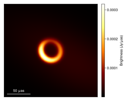
Quantifying the Uncertainty of the Reconstruction
While finding the optimal image is often helpful, in science, the most important thing is to quantify the certainty of our inferences. This is the goal of Comrade. In the language of Bayesian statistics, we want to find a representation of the posterior of possible image reconstructions given our choice of model and the data.
Comrade provides several sampling and other posterior approximation tools. To see the list, please see the Libraries section of the docs. For this example, we will be using Pigeons.jl which is a state-of-the-art parallel tempering sampler that enables global exploration of the posterior. For smaller dimension problems (< 100) we recommend using this sampler, especially if you have access to > 1 core.
using Pigeons
pt = pigeons(target=cpost, explorer=SliceSampler(), record=[traces, round_trip, log_sum_ratio], n_chains=16, n_rounds=8)
PT(checkpoint = false, ...)That's it! To finish it up we can then plot some simple visual fit diagnostics. First we extract the MCMC chain for our posterior.
chain = sample_array(cpost, pt)PosteriorSamples
Samples size: (256,)
sampler used: Pigeons
Mean
┌─────────────────────────────────────────────────────────────────────────────────────────────────────────────────────────────────────────────────────────────────────────────────────────────────────────────────────────────┐
│ sky │
│ @NamedTuple{radius::Float64, width::Float64, ma::Tuple{Float64, Float64}, mp::Tuple{Float64, Float64}, τ::Float64, ξτ::Float64, f::Float64, σG::Float64, τG::Float64, ξG::Float64, xG::Float64, yG::Float64} │
├─────────────────────────────────────────────────────────────────────────────────────────────────────────────────────────────────────────────────────────────────────────────────────────────────────────────────────────────┤
│ (radius = 9.95807e-11, width = 1.88684e-11, ma = (0.28795, 0.0899715), mp = (2.48527, 3.21126), τ = 0.0839587, ξτ = 0.684422, f = 0.298679, σG = 1.4594e-10, τG = 1.56, ξG = 1.51731, xG = -2.25993e-10, yG = -1.12767e-10) │
└─────────────────────────────────────────────────────────────────────────────────────────────────────────────────────────────────────────────────────────────────────────────────────────────────────────────────────────────┘
Std. Dev.
┌────────────────────────────────────────────────────────────────────────────────────────────────────────────────────────────────────────────────────────────────────────────────────────────────────────────────────────────────┐
│ sky │
│ @NamedTuple{radius::Float64, width::Float64, ma::Tuple{Float64, Float64}, mp::Tuple{Float64, Float64}, τ::Float64, ξτ::Float64, f::Float64, σG::Float64, τG::Float64, ξG::Float64, xG::Float64, yG::Float64} │
├────────────────────────────────────────────────────────────────────────────────────────────────────────────────────────────────────────────────────────────────────────────────────────────────────────────────────────────────┤
│ (radius = 1.4152e-12, width = 2.97247e-12, ma = (0.0124975, 0.01645), mp = (0.0340052, 0.219639), τ = 0.025283, ξτ = 0.182928, f = 0.111805, σG = 7.95589e-11, τG = 0.76987, ξG = 0.456943, xG = 4.78689e-11, yG = 2.7743e-11) │
└────────────────────────────────────────────────────────────────────────────────────────────────────────────────────────────────────────────────────────────────────────────────────────────────────────────────────────────────┘First to plot the image we call
imgs = intensitymap.(skymodel.(Ref(post), sample(chain, 100)), Ref(g))
fig = imageviz(imgs[end], colormap=:afmhot)
DisplayAs.Text(DisplayAs.PNG(fig))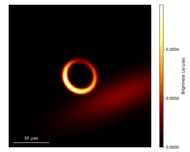
What about the mean image? Well let's grab 100 images from the chain, where we first remove the adaptation steps since they don't sample from the correct posterior distribution
meanimg = mean(imgs)
fig = imageviz(meanimg, colormap=:afmhot);
DisplayAs.Text(DisplayAs.PNG(fig))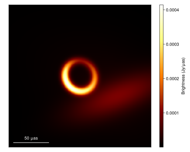
That looks similar to the EHTC VI, and it took us no time at all!. To see how well the model is fitting the data we can plot the model and data products
using Plots
p1 = Plots.plot(simulate_observation(post, xopt; add_thermal_noise=false)[1], label="MAP")
Plots.plot!(p1, dlcamp)
p2 = Plots.plot(simulate_observation(post, xopt; add_thermal_noise=false)[2], label="MAP")
Plots.plot!(p2, dcphase)
DisplayAs.Text(DisplayAs.PNG(Plots.plot(p1, p2, layout=(2,1))))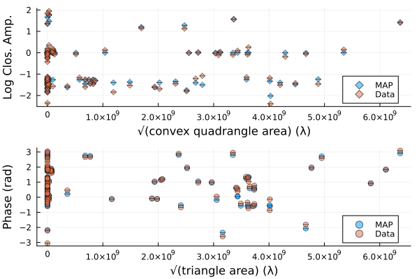
We can also plot random draws from the posterior predictive distribution. The posterior predictive distribution create a number of synthetic observations that are marginalized over the posterior.
p1 = Plots.plot(dlcamp);
p2 = Plots.plot(dcphase);
uva = uvdist.(datatable(dlcamp))
uvp = uvdist.(datatable(dcphase))
for i in 1:10
    mobs = simulate_observation(post, sample(chain, 1)[1])
    mlca = mobs[1]
    mcp  = mobs[2]
    Plots.scatter!(p1, uva, mlca[:measurement], color=:grey, label=:none, alpha=0.2)
    Plots.scatter!(p2, uvp, atan.(sin.(mcp[:measurement]), cos.(mcp[:measurement])), color=:grey, label=:none, alpha=0.2)
end
p = Plots.plot(p1, p2, layout=(2,1));
DisplayAs.Text(DisplayAs.PNG(p))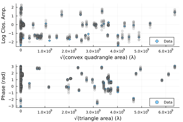
Finally, we can also put everything onto a common scale and plot the normalized residuals. The normalied residuals are the difference between the data and the model, divided by the data's error:
p = residual(post, chain[end]);
DisplayAs.Text(DisplayAs.PNG(p))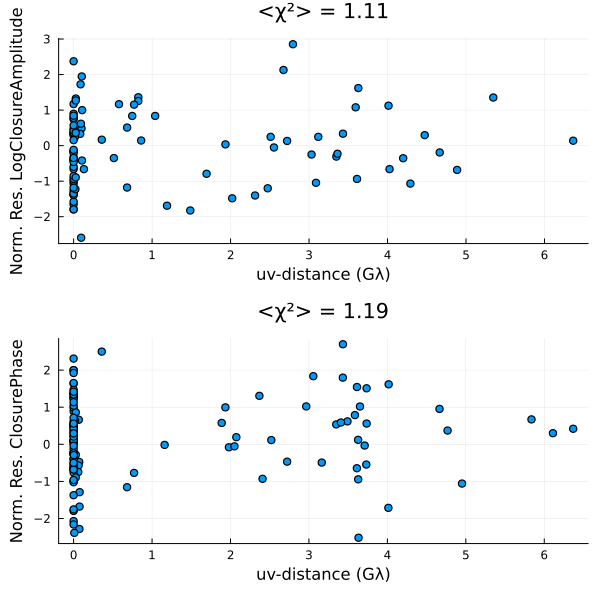
This page was generated using Literate.jl.