Stokes I Simultaneous Image and Instrument Modeling
In this tutorial, we will create a preliminary reconstruction of the 2017 M87 data on April 6 by simultaneously creating an image and model for the instrument. By instrument model, we mean something akin to self-calibration in traditional VLBI imaging terminology. However, unlike traditional self-cal, we will solve for the gains each time we update the image self-consistently. This allows us to model the correlations between gains and the image.
To get started we load Comrade.
using Comrade


using Pyehtim
using LinearAlgebra
CondaPkg Found dependencies: /home/runner/.julia/packages/DimensionalData/bwTLK/CondaPkg.toml
CondaPkg Found dependencies: /home/runner/.julia/packages/PythonCall/WMWY0/CondaPkg.toml
CondaPkg Found dependencies: /home/runner/.julia/packages/Pyehtim/Fm109/CondaPkg.toml
CondaPkg Resolving changes
+ ehtim (pip)
+ libstdcxx-ng
+ numpy
+ numpy (pip)
+ openssl
+ pandas
+ python
+ setuptools (pip)
+ uv
+ xarray
CondaPkg Creating environment
│ /home/runner/.julia/artifacts/7973f2c7725e2d0eef7a95159454c4145f0945a2/bin/micromamba
│ -r /home/runner/.julia/scratchspaces/0b3b1443-0f03-428d-bdfb-f27f9c1191ea/root
│ create
│ -y
│ -p /home/runner/work/Comrade.jl/Comrade.jl/examples/intermediate/StokesIImaging/.CondaPkg/env
│ --override-channels
│ --no-channel-priority
│ libstdcxx-ng[version='>=3.4,<13.0']
│ numpy[version='*']
│ numpy[version='>=1.24, <2.0']
│ openssl[version='>=3, <3.1']
│ pandas[version='<2']
│ python[version='>=3.8,<4',channel='conda-forge',build='*cpython*']
│ python[version='>=3.6,<=3.10']
│ uv[version='>=0.4']
│ xarray[version='*']
└ -c conda-forge
Transaction
Prefix: /home/runner/work/Comrade.jl/Comrade.jl/examples/intermediate/StokesIImaging/.CondaPkg/env
Updating specs:
- libstdcxx-ng[version='>=3.4,<13.0']
- numpy=*
- numpy[version='>=1.24, <2.0']
- openssl[version='>=3, <3.1']
- pandas[version='<2']
- conda-forge::python[version='>=3.8,<4',build=*cpython*]
- python[version='>=3.6,<=3.10']
- uv[version='>=0.4']
- xarray=*
Package Version Build Channel Size
─────────────────────────────────────────────────────────────────────────────────
Install:
─────────────────────────────────────────────────────────────────────────────────
+ libstdcxx-ng 12.3.0 hc0a3c3a_7 conda-forge Cached
+ _libgcc_mutex 0.1 conda_forge conda-forge Cached
+ python_abi 3.10 5_cp310 conda-forge Cached
+ ca-certificates 2024.12.14 hbcca054_0 conda-forge Cached
+ ld_impl_linux-64 2.43 h712a8e2_2 conda-forge Cached
+ libgomp 14.2.0 h77fa898_1 conda-forge Cached
+ _openmp_mutex 4.5 2_gnu conda-forge Cached
+ libgcc 14.2.0 h77fa898_1 conda-forge Cached
+ liblzma 5.6.3 hb9d3cd8_1 conda-forge Cached
+ ncurses 6.5 h2d0b736_3 conda-forge Cached
+ libzlib 1.3.1 hb9d3cd8_2 conda-forge Cached
+ libgfortran5 14.2.0 hd5240d6_1 conda-forge Cached
+ libstdcxx 14.2.0 hc0a3c3a_1 conda-forge Cached
+ libgcc-ng 14.2.0 h69a702a_1 conda-forge Cached
+ xz-tools 5.6.3 hb9d3cd8_1 conda-forge Cached
+ xz-gpl-tools 5.6.3 hbcc6ac9_1 conda-forge Cached
+ liblzma-devel 5.6.3 hb9d3cd8_1 conda-forge Cached
+ libsqlite 3.48.0 hee588c1_1 conda-forge Cached
+ libgfortran 14.2.0 h69a702a_1 conda-forge Cached
+ uv 0.5.25 h0f3a69f_0 conda-forge Cached
+ tk 8.6.13 noxft_h4845f30_101 conda-forge Cached
+ readline 8.2 h8228510_1 conda-forge Cached
+ libuuid 2.38.1 h0b41bf4_0 conda-forge Cached
+ libnsl 2.0.1 hd590300_0 conda-forge Cached
+ libffi 3.4.2 h7f98852_5 conda-forge Cached
+ bzip2 1.0.8 h4bc722e_7 conda-forge Cached
+ openssl 3.0.14 h4ab18f5_0 conda-forge Cached
+ xz 5.6.3 hbcc6ac9_1 conda-forge Cached
+ libopenblas 0.3.28 pthreads_h94d23a6_1 conda-forge Cached
+ sqlite 3.48.0 h9eae976_1 conda-forge Cached
+ libblas 3.9.0 28_h59b9bed_openblas conda-forge Cached
+ libcblas 3.9.0 28_he106b2a_openblas conda-forge Cached
+ liblapack 3.9.0 28_h7ac8fdf_openblas conda-forge Cached
+ tzdata 2025a h78e105d_0 conda-forge Cached
+ python 3.10.0 h543edf9_3_cpython conda-forge Cached
+ wheel 0.45.1 pyhd8ed1ab_1 conda-forge Cached
+ setuptools 75.8.0 pyhff2d567_0 conda-forge Cached
+ pip 25.0 pyh8b19718_0 conda-forge Cached
+ six 1.17.0 pyhd8ed1ab_0 conda-forge Cached
+ pytz 2024.2 pyhd8ed1ab_1 conda-forge Cached
+ packaging 24.2 pyhd8ed1ab_2 conda-forge Cached
+ python-dateutil 2.9.0.post0 pyhff2d567_1 conda-forge Cached
+ numpy 1.26.4 py310hb13e2d6_0 conda-forge Cached
+ pandas 1.5.3 py310h9b08913_1 conda-forge Cached
+ xarray 2024.3.0 pyhd8ed1ab_0 conda-forge Cached
Summary:
Install: 45 packages
Total download: 0 B
─────────────────────────────────────────────────────────────────────────────────
Transaction starting
Linking libstdcxx-ng-12.3.0-hc0a3c3a_7
Linking _libgcc_mutex-0.1-conda_forge
Linking python_abi-3.10-5_cp310
Linking ca-certificates-2024.12.14-hbcca054_0
Linking ld_impl_linux-64-2.43-h712a8e2_2
Linking libgomp-14.2.0-h77fa898_1
Linking _openmp_mutex-4.5-2_gnu
Linking libgcc-14.2.0-h77fa898_1
Linking liblzma-5.6.3-hb9d3cd8_1
Linking ncurses-6.5-h2d0b736_3
Linking libzlib-1.3.1-hb9d3cd8_2
Linking libgfortran5-14.2.0-hd5240d6_1
Linking libstdcxx-14.2.0-hc0a3c3a_1
warning libmamba [libstdcxx-14.2.0-hc0a3c3a_1] The following files were already present in the environment:
- lib/libstdc++.so
- lib/libstdc++.so.6
- share/licenses/libstdc++/RUNTIME.LIBRARY.EXCEPTION
Linking libgcc-ng-14.2.0-h69a702a_1
Linking xz-tools-5.6.3-hb9d3cd8_1
Linking xz-gpl-tools-5.6.3-hbcc6ac9_1
Linking liblzma-devel-5.6.3-hb9d3cd8_1
Linking libsqlite-3.48.0-hee588c1_1
Linking libgfortran-14.2.0-h69a702a_1
Linking uv-0.5.25-h0f3a69f_0
Linking tk-8.6.13-noxft_h4845f30_101
Linking readline-8.2-h8228510_1
Linking libuuid-2.38.1-h0b41bf4_0
Linking libnsl-2.0.1-hd590300_0
Linking libffi-3.4.2-h7f98852_5
Linking bzip2-1.0.8-h4bc722e_7
Linking openssl-3.0.14-h4ab18f5_0
Linking xz-5.6.3-hbcc6ac9_1
Linking libopenblas-0.3.28-pthreads_h94d23a6_1
Linking sqlite-3.48.0-h9eae976_1
Linking libblas-3.9.0-28_h59b9bed_openblas
Linking libcblas-3.9.0-28_he106b2a_openblas
Linking liblapack-3.9.0-28_h7ac8fdf_openblas
Linking tzdata-2025a-h78e105d_0
Linking python-3.10.0-h543edf9_3_cpython
Linking wheel-0.45.1-pyhd8ed1ab_1
Linking setuptools-75.8.0-pyhff2d567_0
Linking pip-25.0-pyh8b19718_0
Linking six-1.17.0-pyhd8ed1ab_0
Linking pytz-2024.2-pyhd8ed1ab_1
Linking packaging-24.2-pyhd8ed1ab_2
Linking python-dateutil-2.9.0.post0-pyhff2d567_1
Linking numpy-1.26.4-py310hb13e2d6_0
Linking pandas-1.5.3-py310h9b08913_1
Linking xarray-2024.3.0-pyhd8ed1ab_0
Transaction finished
To activate this environment, use:
micromamba activate /home/runner/work/Comrade.jl/Comrade.jl/examples/intermediate/StokesIImaging/.CondaPkg/env
Or to execute a single command in this environment, use:
micromamba run -p /home/runner/work/Comrade.jl/Comrade.jl/examples/intermediate/StokesIImaging/.CondaPkg/env mycommand
CondaPkg Installing Pip packages
│ /home/runner/work/Comrade.jl/Comrade.jl/examples/intermediate/StokesIImaging/.CondaPkg/env/bin/uv
│ pip
│ install
│ ehtim >=1.2.10, <2.0
│ numpy >=1.24, <2.0
└ setuptools
Using Python 3.10.0 environment at: /home/runner/work/Comrade.jl/Comrade.jl/examples/intermediate/StokesIImaging/.CondaPkg/env
Resolved 35 packages in 228ms
Installed 29 packages in 73ms
+ astropy==6.1.7
+ astropy-iers-data==0.2025.1.27.0.32.44
+ certifi==2024.12.14
+ charset-normalizer==3.4.1
+ contourpy==1.3.1
+ cycler==0.12.1
+ ehtim==1.2.10
+ fonttools==4.55.8
+ future==1.0.0
+ h5py==3.12.1
+ hdrhistogram==0.10.3
+ idna==3.10
+ jplephem==2.22
+ kiwisolver==1.4.8
+ matplotlib==3.10.0
+ networkx==3.4.2
+ pandas-appender==0.9.9
+ paramsurvey==0.4.21
+ pbr==6.1.0
+ pillow==11.1.0
+ psutil==6.1.1
+ pyerfa==2.0.1.5
+ pyparsing==3.2.1
+ pyyaml==6.0.2
+ requests==2.32.3
+ scipy==1.15.1
+ sgp4==2.23
+ skyfield==1.49
+ urllib3==2.3.0For reproducibility we use a stable random number genreator
using StableRNGs
rng = StableRNG(12)StableRNGs.LehmerRNG(state=0x00000000000000000000000000000019)Load the Data
To download the data visit https://doi.org/10.25739/g85n-f134 First we will load our data:
obs = ehtim.obsdata.load_uvfits(joinpath(__DIR, "..", "..", "Data", "SR1_M87_2017_096_lo_hops_netcal_StokesI.uvfits"))Python: <ehtim.obsdata.Obsdata object at 0x7f03e6679a20>obs = ehtim.obsdata.load_uvfits("~/Dropbox (Smithsonian External)/M872021Project/Data/2021/CASA/e21e18/V4/M87_calibrated_b3.uvf+EVPA_rotation+netcal_10savg+flag.uvfits") Now we do some minor preprocessing:
Scan average the data since the data have been preprocessed so that the gain phases coherent.
Add 1% systematic noise to deal with calibration issues that cause 1% non-closing errors.
obs = scan_average(obs).add_fractional_noise(0.02)Python: <ehtim.obsdata.Obsdata object at 0x7f043772fac0>Now we extract our complex visibilities.
dvis = extract_table(obs, Visibilities())EHTObservationTable{Comrade.EHTVisibilityDatum{:I}}
source: M87
mjd: 57849
bandwidth: 1.856e9
sites: [:AA, :AP, :AZ, :JC, :LM, :PV, :SM]
nsamples: 274##Building the Model/Posterior
Now, we must build our intensity/visibility model. That is, the model that takes in a named tuple of parameters and perhaps some metadata required to construct the model. For our model, we will use a raster or ContinuousImage for our image model. The model is given below:
The model construction is very similar to Imaging a Black Hole using only Closure Quantities, except we include a large scale gaussian since we want to model the zero baselines. For more information about the image model please read the closure-only example.
function sky(θ, metadata)
    (;fg, c, σimg) = θ
    (;ftot, mimg) = metadata
    # Apply the GMRF fluctuations to the image
    rast = apply_fluctuations(CenteredLR(), mimg, σimg.*c.params)
    pimg = parent(rast)
    @. pimg = (ftot*(1-fg))*pimg
    m = ContinuousImage(rast, BSplinePulse{3}())
    x0, y0 = centroid(m)
    # Add a large-scale gaussian to deal with the over-resolved mas flux
    g = modify(Gaussian(), Stretch(μas2rad(500.0), μas2rad(500.0)), Renormalize(ftot*fg))
    return shifted(m, -x0, -y0) + g
end
sky (generic function with 1 method)Now, let's set up our image model. The EHT's nominal resolution is 20-25 μas. Additionally, the EHT is not very sensitive to a larger field of view. Typically 60-80 μas is enough to describe the compact flux of M87. Given this, we only need to use a small number of pixels to describe our image.
npix = 32
fovx = μas2rad(200.0)
fovy = μas2rad(200.0)9.69627362219072e-10Now let's form our cache's. First, we have our usual image cache which is needed to numerically compute the visibilities.
grid = imagepixels(fovx, fovy, npix, npix)RectiGrid(
executor: ComradeBase.Serial()
Dimensions:
(↓ X Sampled{Float64} LinRange{Float64}(-4.69663253574863e-10, 4.69663253574863e-10, 32) ForwardOrdered Regular Points,
→ Y Sampled{Float64} LinRange{Float64}(-4.69663253574863e-10, 4.69663253574863e-10, 32) ForwardOrdered Regular Points)
)Now we need to specify our image prior. For this work we will use a Gaussian Markov Random field prior Since we are using a Gaussian Markov random field prior we need to first specify our mean image. This behaves somewhat similary to a entropy regularizer in that it will start with an initial guess for the image structure. For this tutorial we will use a a symmetric Gaussian with a FWHM of 50 μas
using VLBIImagePriors
using Distributions
fwhmfac = 2*sqrt(2*log(2))
mpr  = modify(Gaussian(), Stretch(μas2rad(50.0)./fwhmfac))
mimg = intensitymap(mpr, grid)
┌ 32×32 IntensityMap{Float64, 2} ┐
├────────────────────────────────┴─────────────────────────────────────── dims ┐
↓ X Sampled{Float64} LinRange{Float64}(-4.69663253574863e-10, 4.69663253574863e-10, 32) ForwardOrdered Regular Points,
→ Y Sampled{Float64} LinRange{Float64}(-4.69663253574863e-10, 4.69663253574863e-10, 32) ForwardOrdered Regular Points
├──────────────────────────────────────────────────────────────────── metadata ┤
ComradeBase.NoHeader()
└──────────────────────────────────────────────────────────────────────────────┘
↓ → -4.69663e-10 -4.39362e-10 -4.09062e-10 -3.78761e-10 -3.4846e-10 -3.18159e-10 -2.87858e-10 -2.57557e-10 -2.27256e-10 -1.96956e-10 -1.66655e-10 -1.36354e-10 -1.06053e-10 -7.57521e-11 -4.54513e-11 -1.51504e-11 1.51504e-11 4.54513e-11 7.57521e-11 1.06053e-10 1.36354e-10 1.66655e-10 1.96956e-10 2.27256e-10 2.57557e-10 2.87858e-10 3.18159e-10 3.4846e-10 3.78761e-10 4.09062e-10 4.39362e-10 4.69663e-10
-4.69663e-10 1.25675e-11 4.60978e-11 1.55054e-10 4.78251e-10 1.3527e-9 3.50847e-9 8.34459e-9 1.81997e-8 3.63993e-8 6.67567e-8 1.12271e-7 1.73145e-7 2.44865e-7 3.1755e-7 3.77633e-7 4.11812e-7 4.11812e-7 3.77633e-7 3.1755e-7 2.44865e-7 1.73145e-7 1.12271e-7 6.67567e-8 3.63993e-8 1.81997e-8 8.34459e-9 3.50847e-9 1.3527e-9 4.78251e-10 1.55054e-10 4.60978e-11 1.25675e-11
-4.39362e-10 4.60978e-11 1.69087e-10 5.6874e-10 1.75423e-9 4.96172e-9 1.28691e-8 3.06081e-8 6.67567e-8 1.33513e-7 2.44865e-7 4.11812e-7 6.351e-7 8.98167e-7 1.16478e-6 1.38516e-6 1.51053e-6 1.51053e-6 1.38516e-6 1.16478e-6 8.98167e-7 6.351e-7 4.11812e-7 2.44865e-7 1.33513e-7 6.67567e-8 3.06081e-8 1.28691e-8 4.96172e-9 1.75423e-9 5.6874e-10 1.69087e-10 4.60978e-11
-4.09062e-10 1.55054e-10 5.6874e-10 1.913e-9 5.90051e-9 1.66892e-8 4.32864e-8 1.02953e-7 2.24542e-7 4.49084e-7 8.23623e-7 1.38516e-6 2.13621e-6 3.02106e-6 3.91783e-6 4.65912e-6 5.0808e-6 5.0808e-6 4.65912e-6 3.91783e-6 3.02106e-6 2.13621e-6 1.38516e-6 8.23623e-7 4.49084e-7 2.24542e-7 1.02953e-7 4.32864e-8 1.66892e-8 5.90051e-9 1.913e-9 5.6874e-10 1.55054e-10
-3.78761e-10 4.78251e-10 1.75423e-9 5.90051e-9 1.81997e-8 5.14764e-8 1.33513e-7 3.1755e-7 6.92582e-7 1.38516e-6 2.5404e-6 4.27243e-6 6.58898e-6 9.31823e-6 1.20843e-5 1.43707e-5 1.56713e-5 1.56713e-5 1.43707e-5 1.20843e-5 9.31823e-6 6.58898e-6 4.27243e-6 2.5404e-6 1.38516e-6 6.92582e-7 3.1755e-7 1.33513e-7 5.14764e-8 1.81997e-8 5.90051e-9 1.75423e-9 4.78251e-10
-3.4846e-10 1.3527e-9 4.96172e-9 1.66892e-8 5.14764e-8 1.45597e-7 3.77633e-7 8.98167e-7 1.95892e-6 3.91783e-6 7.18534e-6 1.20843e-5 1.86365e-5 2.63559e-5 3.41794e-5 4.06464e-5 4.43252e-5 4.43252e-5 4.06464e-5 3.41794e-5 2.63559e-5 1.86365e-5 1.20843e-5 7.18534e-6 3.91783e-6 1.95892e-6 8.98167e-7 3.77633e-7 1.45597e-7 5.14764e-8 1.66892e-8 4.96172e-9 1.3527e-9
-3.18159e-10 3.50847e-9 1.28691e-8 4.32864e-8 1.33513e-7 3.77633e-7 9.79458e-7 2.32956e-6 5.0808e-6 1.01616e-5 1.86365e-5 3.13427e-5 4.8337e-5 6.83588e-5 8.86505e-5 0.000105424 0.000114965 0.000114965 0.000105424 8.86505e-5 6.83588e-5 4.8337e-5 3.13427e-5 1.86365e-5 1.01616e-5 5.0808e-6 2.32956e-6 9.79458e-7 3.77633e-7 1.33513e-7 4.32864e-8 1.28691e-8 3.50847e-9
-2.87858e-10 8.34459e-9 3.06081e-8 1.02953e-7 3.1755e-7 8.98167e-7 2.32956e-6 5.54065e-6 1.20843e-5 2.41685e-5 4.43252e-5 7.45458e-5 0.000114965 0.000162586 0.000210847 0.000250741 0.000273435 0.000273435 0.000250741 0.000210847 0.000162586 0.000114965 7.45458e-5 4.43252e-5 2.41685e-5 1.20843e-5 5.54065e-6 2.32956e-6 8.98167e-7 3.1755e-7 1.02953e-7 3.06081e-8 8.34459e-9
-2.57557e-10 1.81997e-8 6.67567e-8 2.24542e-7 6.92582e-7 1.95892e-6 5.0808e-6 1.20843e-5 2.63559e-5 5.27119e-5 9.6674e-5 0.000162586 0.000250741 0.000354602 0.000459862 0.000546871 0.000596367 0.000596367 0.000546871 0.000459862 0.000354602 0.000250741 0.000162586 9.6674e-5 5.27119e-5 2.63559e-5 1.20843e-5 5.0808e-6 1.95892e-6 6.92582e-7 2.24542e-7 6.67567e-8 1.81997e-8
-2.27256e-10 3.63993e-8 1.33513e-7 4.49084e-7 1.38516e-6 3.91783e-6 1.01616e-5 2.41685e-5 5.27119e-5 0.000105424 0.000193348 0.000325171 0.000501483 0.000709204 0.000919723 0.00109374 0.00119273 0.00119273 0.00109374 0.000919723 0.000709204 0.000501483 0.000325171 0.000193348 0.000105424 5.27119e-5 2.41685e-5 1.01616e-5 3.91783e-6 1.38516e-6 4.49084e-7 1.33513e-7 3.63993e-8
-1.96956e-10 6.67567e-8 2.44865e-7 8.23623e-7 2.5404e-6 7.18534e-6 1.86365e-5 4.43252e-5 9.6674e-5 0.000193348 0.000354602 0.000596367 0.000919723 0.00130069 0.00168678 0.00200593 0.00218748 0.00218748 0.00200593 0.00168678 0.00130069 0.000919723 0.000596367 0.000354602 0.000193348 9.6674e-5 4.43252e-5 1.86365e-5 7.18534e-6 2.5404e-6 8.23623e-7 2.44865e-7 6.67567e-8
-1.66655e-10 1.12271e-7 4.11812e-7 1.38516e-6 4.27243e-6 1.20843e-5 3.13427e-5 7.45458e-5 0.000162586 0.000325171 0.000596367 0.00100297 0.00154678 0.00218748 0.00283681 0.00337356 0.00367889 0.00367889 0.00337356 0.00283681 0.00218748 0.00154678 0.00100297 0.000596367 0.000325171 0.000162586 7.45458e-5 3.13427e-5 1.20843e-5 4.27243e-6 1.38516e-6 4.11812e-7 1.12271e-7
-1.36354e-10 1.73145e-7 6.351e-7 2.13621e-6 6.58898e-6 1.86365e-5 4.8337e-5 0.000114965 0.000250741 0.000501483 0.000919723 0.00154678 0.00238547 0.00337356 0.00437497 0.00520274 0.00567363 0.00567363 0.00520274 0.00437497 0.00337356 0.00238547 0.00154678 0.000919723 0.000501483 0.000250741 0.000114965 4.8337e-5 1.86365e-5 6.58898e-6 2.13621e-6 6.351e-7 1.73145e-7
-1.06053e-10 2.44865e-7 8.98167e-7 3.02106e-6 9.31823e-6 2.63559e-5 6.83588e-5 0.000162586 0.000354602 0.000709204 0.00130069 0.00218748 0.00337356 0.00477093 0.00618714 0.00735779 0.00802372 0.00802372 0.00735779 0.00618714 0.00477093 0.00337356 0.00218748 0.00130069 0.000709204 0.000354602 0.000162586 6.83588e-5 2.63559e-5 9.31823e-6 3.02106e-6 8.98167e-7 2.44865e-7
-7.57521e-11 3.1755e-7 1.16478e-6 3.91783e-6 1.20843e-5 3.41794e-5 8.86505e-5 0.000210847 0.000459862 0.000919723 0.00168678 0.00283681 0.00437497 0.00618714 0.00802372 0.00954187 0.0104055 0.0104055 0.00954187 0.00802372 0.00618714 0.00437497 0.00283681 0.00168678 0.000919723 0.000459862 0.000210847 8.86505e-5 3.41794e-5 1.20843e-5 3.91783e-6 1.16478e-6 3.1755e-7
-4.54513e-11 3.77633e-7 1.38516e-6 4.65912e-6 1.43707e-5 4.06464e-5 0.000105424 0.000250741 0.000546871 0.00109374 0.00200593 0.00337356 0.00520274 0.00735779 0.00954187 0.0113473 0.0123743 0.0123743 0.0113473 0.00954187 0.00735779 0.00520274 0.00337356 0.00200593 0.00109374 0.000546871 0.000250741 0.000105424 4.06464e-5 1.43707e-5 4.65912e-6 1.38516e-6 3.77633e-7
-1.51504e-11 4.11812e-7 1.51053e-6 5.0808e-6 1.56713e-5 4.43252e-5 0.000114965 0.000273435 0.000596367 0.00119273 0.00218748 0.00367889 0.00567363 0.00802372 0.0104055 0.0123743 0.0134942 0.0134942 0.0123743 0.0104055 0.00802372 0.00567363 0.00367889 0.00218748 0.00119273 0.000596367 0.000273435 0.000114965 4.43252e-5 1.56713e-5 5.0808e-6 1.51053e-6 4.11812e-7
1.51504e-11 4.11812e-7 1.51053e-6 5.0808e-6 1.56713e-5 4.43252e-5 0.000114965 0.000273435 0.000596367 0.00119273 0.00218748 0.00367889 0.00567363 0.00802372 0.0104055 0.0123743 0.0134942 0.0134942 0.0123743 0.0104055 0.00802372 0.00567363 0.00367889 0.00218748 0.00119273 0.000596367 0.000273435 0.000114965 4.43252e-5 1.56713e-5 5.0808e-6 1.51053e-6 4.11812e-7
4.54513e-11 3.77633e-7 1.38516e-6 4.65912e-6 1.43707e-5 4.06464e-5 0.000105424 0.000250741 0.000546871 0.00109374 0.00200593 0.00337356 0.00520274 0.00735779 0.00954187 0.0113473 0.0123743 0.0123743 0.0113473 0.00954187 0.00735779 0.00520274 0.00337356 0.00200593 0.00109374 0.000546871 0.000250741 0.000105424 4.06464e-5 1.43707e-5 4.65912e-6 1.38516e-6 3.77633e-7
7.57521e-11 3.1755e-7 1.16478e-6 3.91783e-6 1.20843e-5 3.41794e-5 8.86505e-5 0.000210847 0.000459862 0.000919723 0.00168678 0.00283681 0.00437497 0.00618714 0.00802372 0.00954187 0.0104055 0.0104055 0.00954187 0.00802372 0.00618714 0.00437497 0.00283681 0.00168678 0.000919723 0.000459862 0.000210847 8.86505e-5 3.41794e-5 1.20843e-5 3.91783e-6 1.16478e-6 3.1755e-7
1.06053e-10 2.44865e-7 8.98167e-7 3.02106e-6 9.31823e-6 2.63559e-5 6.83588e-5 0.000162586 0.000354602 0.000709204 0.00130069 0.00218748 0.00337356 0.00477093 0.00618714 0.00735779 0.00802372 0.00802372 0.00735779 0.00618714 0.00477093 0.00337356 0.00218748 0.00130069 0.000709204 0.000354602 0.000162586 6.83588e-5 2.63559e-5 9.31823e-6 3.02106e-6 8.98167e-7 2.44865e-7
1.36354e-10 1.73145e-7 6.351e-7 2.13621e-6 6.58898e-6 1.86365e-5 4.8337e-5 0.000114965 0.000250741 0.000501483 0.000919723 0.00154678 0.00238547 0.00337356 0.00437497 0.00520274 0.00567363 0.00567363 0.00520274 0.00437497 0.00337356 0.00238547 0.00154678 0.000919723 0.000501483 0.000250741 0.000114965 4.8337e-5 1.86365e-5 6.58898e-6 2.13621e-6 6.351e-7 1.73145e-7
1.66655e-10 1.12271e-7 4.11812e-7 1.38516e-6 4.27243e-6 1.20843e-5 3.13427e-5 7.45458e-5 0.000162586 0.000325171 0.000596367 0.00100297 0.00154678 0.00218748 0.00283681 0.00337356 0.00367889 0.00367889 0.00337356 0.00283681 0.00218748 0.00154678 0.00100297 0.000596367 0.000325171 0.000162586 7.45458e-5 3.13427e-5 1.20843e-5 4.27243e-6 1.38516e-6 4.11812e-7 1.12271e-7
1.96956e-10 6.67567e-8 2.44865e-7 8.23623e-7 2.5404e-6 7.18534e-6 1.86365e-5 4.43252e-5 9.6674e-5 0.000193348 0.000354602 0.000596367 0.000919723 0.00130069 0.00168678 0.00200593 0.00218748 0.00218748 0.00200593 0.00168678 0.00130069 0.000919723 0.000596367 0.000354602 0.000193348 9.6674e-5 4.43252e-5 1.86365e-5 7.18534e-6 2.5404e-6 8.23623e-7 2.44865e-7 6.67567e-8
2.27256e-10 3.63993e-8 1.33513e-7 4.49084e-7 1.38516e-6 3.91783e-6 1.01616e-5 2.41685e-5 5.27119e-5 0.000105424 0.000193348 0.000325171 0.000501483 0.000709204 0.000919723 0.00109374 0.00119273 0.00119273 0.00109374 0.000919723 0.000709204 0.000501483 0.000325171 0.000193348 0.000105424 5.27119e-5 2.41685e-5 1.01616e-5 3.91783e-6 1.38516e-6 4.49084e-7 1.33513e-7 3.63993e-8
2.57557e-10 1.81997e-8 6.67567e-8 2.24542e-7 6.92582e-7 1.95892e-6 5.0808e-6 1.20843e-5 2.63559e-5 5.27119e-5 9.6674e-5 0.000162586 0.000250741 0.000354602 0.000459862 0.000546871 0.000596367 0.000596367 0.000546871 0.000459862 0.000354602 0.000250741 0.000162586 9.6674e-5 5.27119e-5 2.63559e-5 1.20843e-5 5.0808e-6 1.95892e-6 6.92582e-7 2.24542e-7 6.67567e-8 1.81997e-8
2.87858e-10 8.34459e-9 3.06081e-8 1.02953e-7 3.1755e-7 8.98167e-7 2.32956e-6 5.54065e-6 1.20843e-5 2.41685e-5 4.43252e-5 7.45458e-5 0.000114965 0.000162586 0.000210847 0.000250741 0.000273435 0.000273435 0.000250741 0.000210847 0.000162586 0.000114965 7.45458e-5 4.43252e-5 2.41685e-5 1.20843e-5 5.54065e-6 2.32956e-6 8.98167e-7 3.1755e-7 1.02953e-7 3.06081e-8 8.34459e-9
3.18159e-10 3.50847e-9 1.28691e-8 4.32864e-8 1.33513e-7 3.77633e-7 9.79458e-7 2.32956e-6 5.0808e-6 1.01616e-5 1.86365e-5 3.13427e-5 4.8337e-5 6.83588e-5 8.86505e-5 0.000105424 0.000114965 0.000114965 0.000105424 8.86505e-5 6.83588e-5 4.8337e-5 3.13427e-5 1.86365e-5 1.01616e-5 5.0808e-6 2.32956e-6 9.79458e-7 3.77633e-7 1.33513e-7 4.32864e-8 1.28691e-8 3.50847e-9
3.4846e-10 1.3527e-9 4.96172e-9 1.66892e-8 5.14764e-8 1.45597e-7 3.77633e-7 8.98167e-7 1.95892e-6 3.91783e-6 7.18534e-6 1.20843e-5 1.86365e-5 2.63559e-5 3.41794e-5 4.06464e-5 4.43252e-5 4.43252e-5 4.06464e-5 3.41794e-5 2.63559e-5 1.86365e-5 1.20843e-5 7.18534e-6 3.91783e-6 1.95892e-6 8.98167e-7 3.77633e-7 1.45597e-7 5.14764e-8 1.66892e-8 4.96172e-9 1.3527e-9
3.78761e-10 4.78251e-10 1.75423e-9 5.90051e-9 1.81997e-8 5.14764e-8 1.33513e-7 3.1755e-7 6.92582e-7 1.38516e-6 2.5404e-6 4.27243e-6 6.58898e-6 9.31823e-6 1.20843e-5 1.43707e-5 1.56713e-5 1.56713e-5 1.43707e-5 1.20843e-5 9.31823e-6 6.58898e-6 4.27243e-6 2.5404e-6 1.38516e-6 6.92582e-7 3.1755e-7 1.33513e-7 5.14764e-8 1.81997e-8 5.90051e-9 1.75423e-9 4.78251e-10
4.09062e-10 1.55054e-10 5.6874e-10 1.913e-9 5.90051e-9 1.66892e-8 4.32864e-8 1.02953e-7 2.24542e-7 4.49084e-7 8.23623e-7 1.38516e-6 2.13621e-6 3.02106e-6 3.91783e-6 4.65912e-6 5.0808e-6 5.0808e-6 4.65912e-6 3.91783e-6 3.02106e-6 2.13621e-6 1.38516e-6 8.23623e-7 4.49084e-7 2.24542e-7 1.02953e-7 4.32864e-8 1.66892e-8 5.90051e-9 1.913e-9 5.6874e-10 1.55054e-10
4.39362e-10 4.60978e-11 1.69087e-10 5.6874e-10 1.75423e-9 4.96172e-9 1.28691e-8 3.06081e-8 6.67567e-8 1.33513e-7 2.44865e-7 4.11812e-7 6.351e-7 8.98167e-7 1.16478e-6 1.38516e-6 1.51053e-6 1.51053e-6 1.38516e-6 1.16478e-6 8.98167e-7 6.351e-7 4.11812e-7 2.44865e-7 1.33513e-7 6.67567e-8 3.06081e-8 1.28691e-8 4.96172e-9 1.75423e-9 5.6874e-10 1.69087e-10 4.60978e-11
4.69663e-10 1.25675e-11 4.60978e-11 1.55054e-10 4.78251e-10 1.3527e-9 3.50847e-9 8.34459e-9 1.81997e-8 3.63993e-8 6.67567e-8 1.12271e-7 1.73145e-7 2.44865e-7 3.1755e-7 3.77633e-7 4.11812e-7 4.11812e-7 3.77633e-7 3.1755e-7 2.44865e-7 1.73145e-7 1.12271e-7 6.67567e-8 3.63993e-8 1.81997e-8 8.34459e-9 3.50847e-9 1.3527e-9 4.78251e-10 1.55054e-10 4.60978e-11 1.25675e-11Now we can form our metadata we need to fully define our model. We will also fix the total flux to be the observed value 1.1. This is because total flux is degenerate with a global shift in the gain amplitudes making the problem degenerate. To fix this we use the observed total flux as our value.
skymeta = (;ftot = 1.1, mimg = mimg./flux(mimg))(ftot = 1.1, mimg = [1.2567547416996487e-11 4.60979671782088e-11 1.5505446140255663e-10 4.782533378056425e-10 1.3527047131498763e-9 3.5084819555512232e-9 8.344623408800353e-9 1.8199752706952592e-8 3.639950541390525e-8 6.675698727040275e-8 1.1227142257763898e-7 1.7314620328318453e-7 2.448657089564883e-7 3.175515369524363e-7 3.7763454712388683e-7 4.1181339376014135e-7 4.1181339376014135e-7 3.7763454712388683e-7 3.175515369524363e-7 2.448657089564883e-7 1.7314620328318453e-7 1.1227142257763922e-7 6.675698727040275e-8 3.639950541390525e-8 1.8199752706952592e-8 8.344623408800353e-9 3.5084819555512232e-9 1.3527047131498763e-9 4.782533378056425e-10 1.5505446140255717e-10 4.60979671782088e-11 1.2567547416996487e-11; 4.60979671782088e-11 1.690880891437348e-10 5.687422720922681e-10 1.7542409777756147e-9 4.9617427648818055e-9 1.2869168555004412e-8 3.060821361956108e-8 6.675698727040275e-8 1.335139745408057e-7 2.448657089564883e-7 4.1181339376014066e-7 6.351030739048726e-7 8.981713806211123e-7 1.1647841732449665e-6 1.3851696262654769e-6 1.510538188495548e-6 1.510538188495548e-6 1.3851696262654769e-6 1.1647841732449665e-6 8.981713806211123e-7 6.351030739048726e-7 4.1181339376014135e-7 2.448657089564883e-7 1.335139745408057e-7 6.675698727040275e-8 3.060821361956108e-8 1.2869168555004412e-8 4.9617427648818055e-9 1.7542409777756147e-9 5.687422720922701e-10 1.690880891437348e-10 4.60979671782088e-11; 1.5505446140255663e-10 5.687422720922681e-10 1.913013351222567e-9 5.900539798810739e-9 1.6689246817600684e-8 4.328655082079613e-8 1.0295334844003551e-7 2.2454284515527802e-7 4.4908569031055694e-7 8.23626787520283e-7 1.3851696262654769e-6 2.136223592652892e-6 3.021076376991096e-6 3.917851343303821e-6 4.659136692979867e-6 5.0808245912389815e-6 5.0808245912389815e-6 4.659136692979867e-6 3.917851343303814e-6 3.021076376991096e-6 2.136223592652892e-6 1.3851696262654794e-6 8.236267875202814e-7 4.4908569031055694e-7 2.2454284515527802e-7 1.0295334844003551e-7 4.328655082079613e-8 1.6689246817600684e-8 5.900539798810739e-9 1.9130133512225742e-9 5.687422720922681e-10 1.5505446140255663e-10; 4.782533378056425e-10 1.7542409777756147e-9 5.900539798810739e-9 1.819975270695265e-8 5.1476674220017655e-8 1.3351397454080597e-7 3.175515369524369e-7 6.925848131327384e-7 1.3851696262654794e-6 2.5404122956194908e-6 4.272447185305786e-6 6.589014300162271e-6 9.318273385959749e-6 1.2084305507964394e-5 1.4370742089937826e-5 1.5671405373215287e-5 1.5671405373215287e-5 1.4370742089937826e-5 1.2084305507964394e-5 9.318273385959749e-6 6.589014300162271e-6 4.272447185305794e-6 2.5404122956194908e-6 1.3851696262654794e-6 6.925848131327384e-7 3.175515369524369e-7 1.3351397454080597e-7 5.1476674220017655e-8 1.819975270695265e-8 5.90053979881076e-9 1.7542409777756147e-9 4.782533378056425e-10; 1.3527047131498763e-9 4.9617427648818055e-9 1.6689246817600684e-8 5.1476674220017655e-8 1.455980216556205e-7 3.7763454712388614e-7 8.981713806211139e-7 1.9589256716519037e-6 3.917851343303814e-6 7.185371044968894e-6 1.2084305507964365e-5 1.8636546771919454e-5 2.6356057200649016e-5 3.41795774824462e-5 4.0646596729911805e-5 4.432542804049519e-5 4.432542804049519e-5 4.0646596729911805e-5 3.41795774824462e-5 2.6356057200649016e-5 1.8636546771919454e-5 1.2084305507964374e-5 7.185371044968885e-6 3.917851343303814e-6 1.9589256716519037e-6 8.981713806211139e-7 3.7763454712388614e-7 1.455980216556205e-7 5.1476674220017655e-8 1.6689246817600743e-8 4.9617427648818055e-9 1.3527047131498763e-9; 3.5084819555512232e-9 1.2869168555004412e-8 4.328655082079613e-8 1.3351397454080597e-7 3.7763454712388614e-7 9.79462835825955e-7 2.329568346489937e-6 5.0808245912389815e-6 1.0161649182477983e-5 1.863654677191947e-5 3.134281074643055e-5 4.833722203185754e-5 6.835915496489247e-5 8.865085608099055e-5 0.00010542422880259616 0.00011496593671950256 0.00011496593671950256 0.00010542422880259628 8.865085608099055e-5 6.835915496489247e-5 4.833722203185754e-5 3.1342810746430575e-5 1.863654677191947e-5 1.0161649182477983e-5 5.0808245912389815e-6 2.329568346489937e-6 9.79462835825955e-7 3.7763454712388614e-7 1.3351397454080597e-7 4.3286550820796285e-8 1.2869168555004412e-8 3.5084819555512232e-9; 8.344623408800353e-9 3.060821361956108e-8 1.0295334844003551e-7 3.175515369524369e-7 8.981713806211139e-7 2.329568346489937e-6 5.540678505061918e-6 1.2084305507964385e-5 2.4168611015928815e-5 4.4325428040495274e-5 7.454618708767795e-5 0.00011496593671950265 0.0001625863869196475 0.0002108484576051926 0.0002507424859714445 0.00027343661985957014 0.00027343661985957014 0.0002507424859714447 0.0002108484576051926 0.0001625863869196475 0.00011496593671950265 7.454618708767802e-5 4.4325428040495274e-5 2.4168611015928815e-5 1.2084305507964385e-5 5.540678505061918e-6 2.329568346489937e-6 8.981713806211139e-7 3.175515369524369e-7 1.0295334844003588e-7 3.060821361956108e-8 8.344623408800353e-9; 1.8199752706952592e-8 6.675698727040275e-8 2.2454284515527802e-7 6.925848131327384e-7 1.9589256716519037e-6 5.0808245912389815e-6 1.2084305507964385e-5 2.6356057200648992e-5 5.271211440129808e-5 9.667444406371495e-5 0.00016258638691964722 0.00025074248597144427 0.0003546034243239617 0.0004598637468780097 0.0005468732397191394 0.0005963694967014225 0.0005963694967014225 0.0005468732397191394 0.0004598637468780094 0.0003546034243239617 0.00025074248597144427 0.0001625863869196475 9.667444406371485e-5 5.271211440129808e-5 2.6356057200648992e-5 1.2084305507964385e-5 5.0808245912389815e-6 1.9589256716519037e-6 6.925848131327384e-7 2.2454284515527882e-7 6.675698727040275e-8 1.8199752706952592e-8; 3.639950541390525e-8 1.335139745408057e-7 4.4908569031055694e-7 1.3851696262654794e-6 3.917851343303814e-6 1.0161649182477983e-5 2.4168611015928815e-5 5.271211440129808e-5 0.00010542422880259636 0.00019334888812743022 0.000325172773839295 0.0005014849719428892 0.0007092068486479246 0.0009197274937560213 0.0010937464794382808 0.0011927389934028472 0.0011927389934028472 0.0010937464794382808 0.0009197274937560206 0.0007092068486479246 0.0005014849719428892 0.0003251727738392957 0.00019334888812743006 0.00010542422880259636 5.271211440129808e-5 2.4168611015928815e-5 1.0161649182477983e-5 3.917851343303814e-6 1.3851696262654794e-6 4.490856903105585e-7 1.335139745408057e-7 3.639950541390525e-8; 6.675698727040275e-8 2.448657089564883e-7 8.23626787520283e-7 2.5404122956194908e-6 7.185371044968894e-6 1.863654677191947e-5 4.4325428040495274e-5 9.667444406371495e-5 0.00019334888812743022 0.0003546034243239617 0.0005963694967014229 0.0009197274937560198 0.0013006910953571786 0.001686787660841538 0.0020059398877715537 0.002187492958876558 0.002187492958876558 0.0020059398877715537 0.0016867876608415372 0.0013006910953571786 0.0009197274937560198 0.0005963694967014233 0.00035460342432396154 0.00019334888812743022 9.667444406371495e-5 4.4325428040495274e-5 1.863654677191947e-5 7.185371044968894e-6 2.5404122956194908e-6 8.23626787520286e-7 2.448657089564883e-7 6.675698727040275e-8; 1.1227142257763898e-7 4.1181339376014066e-7 1.3851696262654769e-6 4.272447185305786e-6 1.2084305507964365e-5 3.134281074643055e-5 7.454618708767795e-5 0.00016258638691964722 0.000325172773839295 0.0005963694967014229 0.0010029699438857767 0.0015467911050194411 0.002187492958876558 0.0028368273945916967 0.0033735753216830766 0.003678909975024079 0.003678909975024079 0.0033735753216830766 0.0028368273945916954 0.002187492958876558 0.0015467911050194411 0.001002969943885778 0.0005963694967014221 0.000325172773839295 0.00016258638691964722 7.454618708767795e-5 3.134281074643055e-5 1.2084305507964365e-5 4.272447185305786e-6 1.3851696262654818e-6 4.1181339376014066e-7 1.1227142257763898e-7; 1.7314620328318453e-7 6.351030739048726e-7 2.136223592652892e-6 6.589014300162271e-6 1.8636546771919454e-5 4.833722203185754e-5 0.00011496593671950265 0.00025074248597144427 0.0005014849719428892 0.0009197274937560198 0.0015467911050194411 0.002385477986805694 0.003373575321683077 0.004374985917753121 0.00520276438142872 0.005673654789183394 0.005673654789183394 0.00520276438142872 0.004374985917753119 0.003373575321683077 0.002385477986805694 0.0015467911050194428 0.0009197274937560193 0.0005014849719428892 0.00025074248597144427 0.00011496593671950265 4.833722203185754e-5 1.8636546771919454e-5 6.589014300162271e-6 2.1362235926529e-6 6.351030739048726e-7 1.7314620328318453e-7; 2.448657089564883e-7 8.981713806211123e-7 3.021076376991096e-6 9.318273385959749e-6 2.6356057200649016e-5 6.835915496489247e-5 0.0001625863869196475 0.0003546034243239617 0.0007092068486479246 0.0013006910953571786 0.002187492958876558 0.003373575321683077 0.004770955973611384 0.006187164420077763 0.007357819950048159 0.008023759551086217 0.008023759551086217 0.007357819950048159 0.006187164420077759 0.004770955973611384 0.003373575321683077 0.002187492958876561 0.001300691095357178 0.0007092068486479246 0.0003546034243239617 0.0001625863869196475 6.835915496489247e-5 2.6356057200649016e-5 9.318273385959749e-6 3.0210763769911065e-6 8.981713806211123e-7 2.448657089564883e-7; 3.175515369524363e-7 1.1647841732449665e-6 3.917851343303821e-6 1.2084305507964394e-5 3.41795774824462e-5 8.865085608099055e-5 0.0002108484576051926 0.0004598637468780097 0.0009197274937560213 0.001686787660841538 0.0028368273945916967 0.004374985917753121 0.006187164420077763 0.008023759551086224 0.009541911947222773 0.010405528762857438 0.010405528762857438 0.009541911947222773 0.008023759551086218 0.006187164420077763 0.004374985917753121 0.002836827394591701 0.001686787660841538 0.0009197274937560213 0.0004598637468780097 0.0002108484576051926 8.865085608099055e-5 3.41795774824462e-5 1.2084305507964394e-5 3.917851343303835e-6 1.1647841732449665e-6 3.175515369524363e-7; 3.7763454712388683e-7 1.3851696262654769e-6 4.659136692979867e-6 1.4370742089937826e-5 4.0646596729911805e-5 0.00010542422880259616 0.0002507424859714445 0.0005468732397191394 0.0010937464794382808 0.0020059398877715537 0.0033735753216830766 0.00520276438142872 0.007357819950048159 0.009541911947222773 0.011347309578366787 0.012374328840155524 0.012374328840155524 0.011347309578366787 0.009541911947222767 0.007357819950048159 0.00520276438142872 0.0033735753216830814 0.0020059398877715524 0.0010937464794382808 0.0005468732397191394 0.0002507424859714445 0.00010542422880259616 4.0646596729911805e-5 1.4370742089937826e-5 4.659136692979882e-6 1.3851696262654769e-6 3.7763454712388683e-7; 4.1181339376014135e-7 1.510538188495548e-6 5.0808245912389815e-6 1.5671405373215287e-5 4.432542804049519e-5 0.00011496593671950256 0.00027343661985957014 0.0005963694967014225 0.0011927389934028472 0.002187492958876558 0.003678909975024079 0.005673654789183394 0.008023759551086217 0.010405528762857438 0.012374328840155524 0.013494301286732307 0.013494301286732307 0.012374328840155525 0.010405528762857434 0.008023759551086217 0.005673654789183394 0.0036789099750240833 0.0021874929588765572 0.0011927389934028472 0.0005963694967014225 0.00027343661985957014 0.00011496593671950256 4.432542804049519e-5 1.5671405373215287e-5 5.080824591239e-6 1.510538188495548e-6 4.1181339376014135e-7; 4.1181339376014135e-7 1.510538188495548e-6 5.0808245912389815e-6 1.5671405373215287e-5 4.432542804049519e-5 0.00011496593671950256 0.00027343661985957014 0.0005963694967014225 0.0011927389934028472 0.002187492958876558 0.003678909975024079 0.005673654789183394 0.008023759551086217 0.010405528762857438 0.012374328840155524 0.013494301286732307 0.013494301286732307 0.012374328840155525 0.010405528762857434 0.008023759551086217 0.005673654789183394 0.0036789099750240833 0.0021874929588765572 0.0011927389934028472 0.0005963694967014225 0.00027343661985957014 0.00011496593671950256 4.432542804049519e-5 1.5671405373215287e-5 5.080824591239e-6 1.510538188495548e-6 4.1181339376014135e-7; 3.7763454712388683e-7 1.3851696262654769e-6 4.659136692979867e-6 1.4370742089937826e-5 4.0646596729911805e-5 0.00010542422880259628 0.0002507424859714447 0.0005468732397191394 0.0010937464794382808 0.0020059398877715537 0.0033735753216830766 0.00520276438142872 0.007357819950048159 0.009541911947222773 0.011347309578366787 0.012374328840155525 0.012374328840155525 0.011347309578366788 0.009541911947222769 0.007357819950048159 0.00520276438142872 0.0033735753216830814 0.0020059398877715524 0.0010937464794382808 0.0005468732397191394 0.0002507424859714447 0.00010542422880259628 4.0646596729911805e-5 1.4370742089937826e-5 4.659136692979882e-6 1.3851696262654769e-6 3.7763454712388683e-7; 3.175515369524363e-7 1.1647841732449665e-6 3.917851343303814e-6 1.2084305507964394e-5 3.41795774824462e-5 8.865085608099055e-5 0.0002108484576051926 0.0004598637468780094 0.0009197274937560206 0.0016867876608415372 0.0028368273945916954 0.004374985917753119 0.006187164420077759 0.008023759551086218 0.009541911947222767 0.010405528762857434 0.010405528762857434 0.009541911947222769 0.008023759551086213 0.006187164420077759 0.004374985917753119 0.0028368273945916997 0.0016867876608415364 0.0009197274937560206 0.0004598637468780094 0.0002108484576051926 8.865085608099055e-5 3.41795774824462e-5 1.2084305507964394e-5 3.917851343303829e-6 1.1647841732449665e-6 3.175515369524363e-7; 2.448657089564883e-7 8.981713806211123e-7 3.021076376991096e-6 9.318273385959749e-6 2.6356057200649016e-5 6.835915496489247e-5 0.0001625863869196475 0.0003546034243239617 0.0007092068486479246 0.0013006910953571786 0.002187492958876558 0.003373575321683077 0.004770955973611384 0.006187164420077763 0.007357819950048159 0.008023759551086217 0.008023759551086217 0.007357819950048159 0.006187164420077759 0.004770955973611384 0.003373575321683077 0.002187492958876561 0.001300691095357178 0.0007092068486479246 0.0003546034243239617 0.0001625863869196475 6.835915496489247e-5 2.6356057200649016e-5 9.318273385959749e-6 3.0210763769911065e-6 8.981713806211123e-7 2.448657089564883e-7; 1.7314620328318453e-7 6.351030739048726e-7 2.136223592652892e-6 6.589014300162271e-6 1.8636546771919454e-5 4.833722203185754e-5 0.00011496593671950265 0.00025074248597144427 0.0005014849719428892 0.0009197274937560198 0.0015467911050194411 0.002385477986805694 0.003373575321683077 0.004374985917753121 0.00520276438142872 0.005673654789183394 0.005673654789183394 0.00520276438142872 0.004374985917753119 0.003373575321683077 0.002385477986805694 0.0015467911050194428 0.0009197274937560193 0.0005014849719428892 0.00025074248597144427 0.00011496593671950265 4.833722203185754e-5 1.8636546771919454e-5 6.589014300162271e-6 2.1362235926529e-6 6.351030739048726e-7 1.7314620328318453e-7; 1.1227142257763922e-7 4.1181339376014135e-7 1.3851696262654794e-6 4.272447185305794e-6 1.2084305507964374e-5 3.1342810746430575e-5 7.454618708767802e-5 0.0001625863869196475 0.0003251727738392957 0.0005963694967014233 0.001002969943885778 0.0015467911050194428 0.002187492958876561 0.002836827394591701 0.0033735753216830814 0.0036789099750240833 0.0036789099750240833 0.0033735753216830814 0.0028368273945916997 0.002187492958876561 0.0015467911050194428 0.0010029699438857793 0.0005963694967014233 0.0003251727738392957 0.0001625863869196475 7.454618708767802e-5 3.1342810746430575e-5 1.2084305507964374e-5 4.272447185305794e-6 1.3851696262654843e-6 4.1181339376014135e-7 1.1227142257763922e-7; 6.675698727040275e-8 2.448657089564883e-7 8.236267875202814e-7 2.5404122956194908e-6 7.185371044968885e-6 1.863654677191947e-5 4.4325428040495274e-5 9.667444406371485e-5 0.00019334888812743006 0.00035460342432396154 0.0005963694967014221 0.0009197274937560193 0.001300691095357178 0.001686787660841538 0.0020059398877715524 0.0021874929588765572 0.0021874929588765572 0.0020059398877715524 0.0016867876608415364 0.001300691095357178 0.0009197274937560193 0.0005963694967014233 0.0003546034243239614 0.00019334888812743006 9.667444406371485e-5 4.4325428040495274e-5 1.863654677191947e-5 7.185371044968885e-6 2.5404122956194908e-6 8.236267875202844e-7 2.448657089564883e-7 6.675698727040275e-8; 3.639950541390525e-8 1.335139745408057e-7 4.4908569031055694e-7 1.3851696262654794e-6 3.917851343303814e-6 1.0161649182477983e-5 2.4168611015928815e-5 5.271211440129808e-5 0.00010542422880259636 0.00019334888812743022 0.000325172773839295 0.0005014849719428892 0.0007092068486479246 0.0009197274937560213 0.0010937464794382808 0.0011927389934028472 0.0011927389934028472 0.0010937464794382808 0.0009197274937560206 0.0007092068486479246 0.0005014849719428892 0.0003251727738392957 0.00019334888812743006 0.00010542422880259636 5.271211440129808e-5 2.4168611015928815e-5 1.0161649182477983e-5 3.917851343303814e-6 1.3851696262654794e-6 4.490856903105585e-7 1.335139745408057e-7 3.639950541390525e-8; 1.8199752706952592e-8 6.675698727040275e-8 2.2454284515527802e-7 6.925848131327384e-7 1.9589256716519037e-6 5.0808245912389815e-6 1.2084305507964385e-5 2.6356057200648992e-5 5.271211440129808e-5 9.667444406371495e-5 0.00016258638691964722 0.00025074248597144427 0.0003546034243239617 0.0004598637468780097 0.0005468732397191394 0.0005963694967014225 0.0005963694967014225 0.0005468732397191394 0.0004598637468780094 0.0003546034243239617 0.00025074248597144427 0.0001625863869196475 9.667444406371485e-5 5.271211440129808e-5 2.6356057200648992e-5 1.2084305507964385e-5 5.0808245912389815e-6 1.9589256716519037e-6 6.925848131327384e-7 2.2454284515527882e-7 6.675698727040275e-8 1.8199752706952592e-8; 8.344623408800353e-9 3.060821361956108e-8 1.0295334844003551e-7 3.175515369524369e-7 8.981713806211139e-7 2.329568346489937e-6 5.540678505061918e-6 1.2084305507964385e-5 2.4168611015928815e-5 4.4325428040495274e-5 7.454618708767795e-5 0.00011496593671950265 0.0001625863869196475 0.0002108484576051926 0.0002507424859714445 0.00027343661985957014 0.00027343661985957014 0.0002507424859714447 0.0002108484576051926 0.0001625863869196475 0.00011496593671950265 7.454618708767802e-5 4.4325428040495274e-5 2.4168611015928815e-5 1.2084305507964385e-5 5.540678505061918e-6 2.329568346489937e-6 8.981713806211139e-7 3.175515369524369e-7 1.0295334844003588e-7 3.060821361956108e-8 8.344623408800353e-9; 3.5084819555512232e-9 1.2869168555004412e-8 4.328655082079613e-8 1.3351397454080597e-7 3.7763454712388614e-7 9.79462835825955e-7 2.329568346489937e-6 5.0808245912389815e-6 1.0161649182477983e-5 1.863654677191947e-5 3.134281074643055e-5 4.833722203185754e-5 6.835915496489247e-5 8.865085608099055e-5 0.00010542422880259616 0.00011496593671950256 0.00011496593671950256 0.00010542422880259628 8.865085608099055e-5 6.835915496489247e-5 4.833722203185754e-5 3.1342810746430575e-5 1.863654677191947e-5 1.0161649182477983e-5 5.0808245912389815e-6 2.329568346489937e-6 9.79462835825955e-7 3.7763454712388614e-7 1.3351397454080597e-7 4.3286550820796285e-8 1.2869168555004412e-8 3.5084819555512232e-9; 1.3527047131498763e-9 4.9617427648818055e-9 1.6689246817600684e-8 5.1476674220017655e-8 1.455980216556205e-7 3.7763454712388614e-7 8.981713806211139e-7 1.9589256716519037e-6 3.917851343303814e-6 7.185371044968894e-6 1.2084305507964365e-5 1.8636546771919454e-5 2.6356057200649016e-5 3.41795774824462e-5 4.0646596729911805e-5 4.432542804049519e-5 4.432542804049519e-5 4.0646596729911805e-5 3.41795774824462e-5 2.6356057200649016e-5 1.8636546771919454e-5 1.2084305507964374e-5 7.185371044968885e-6 3.917851343303814e-6 1.9589256716519037e-6 8.981713806211139e-7 3.7763454712388614e-7 1.455980216556205e-7 5.1476674220017655e-8 1.6689246817600743e-8 4.9617427648818055e-9 1.3527047131498763e-9; 4.782533378056425e-10 1.7542409777756147e-9 5.900539798810739e-9 1.819975270695265e-8 5.1476674220017655e-8 1.3351397454080597e-7 3.175515369524369e-7 6.925848131327384e-7 1.3851696262654794e-6 2.5404122956194908e-6 4.272447185305786e-6 6.589014300162271e-6 9.318273385959749e-6 1.2084305507964394e-5 1.4370742089937826e-5 1.5671405373215287e-5 1.5671405373215287e-5 1.4370742089937826e-5 1.2084305507964394e-5 9.318273385959749e-6 6.589014300162271e-6 4.272447185305794e-6 2.5404122956194908e-6 1.3851696262654794e-6 6.925848131327384e-7 3.175515369524369e-7 1.3351397454080597e-7 5.1476674220017655e-8 1.819975270695265e-8 5.90053979881076e-9 1.7542409777756147e-9 4.782533378056425e-10; 1.5505446140255717e-10 5.687422720922701e-10 1.9130133512225742e-9 5.90053979881076e-9 1.6689246817600743e-8 4.3286550820796285e-8 1.0295334844003588e-7 2.2454284515527882e-7 4.490856903105585e-7 8.23626787520286e-7 1.3851696262654818e-6 2.1362235926529e-6 3.0210763769911065e-6 3.917851343303835e-6 4.659136692979882e-6 5.080824591239e-6 5.080824591239e-6 4.659136692979882e-6 3.917851343303829e-6 3.0210763769911065e-6 2.1362235926529e-6 1.3851696262654843e-6 8.236267875202844e-7 4.490856903105585e-7 2.2454284515527882e-7 1.0295334844003588e-7 4.3286550820796285e-8 1.6689246817600743e-8 5.90053979881076e-9 1.913013351222581e-9 5.687422720922701e-10 1.5505446140255717e-10; 4.60979671782088e-11 1.690880891437348e-10 5.687422720922681e-10 1.7542409777756147e-9 4.9617427648818055e-9 1.2869168555004412e-8 3.060821361956108e-8 6.675698727040275e-8 1.335139745408057e-7 2.448657089564883e-7 4.1181339376014066e-7 6.351030739048726e-7 8.981713806211123e-7 1.1647841732449665e-6 1.3851696262654769e-6 1.510538188495548e-6 1.510538188495548e-6 1.3851696262654769e-6 1.1647841732449665e-6 8.981713806211123e-7 6.351030739048726e-7 4.1181339376014135e-7 2.448657089564883e-7 1.335139745408057e-7 6.675698727040275e-8 3.060821361956108e-8 1.2869168555004412e-8 4.9617427648818055e-9 1.7542409777756147e-9 5.687422720922701e-10 1.690880891437348e-10 4.60979671782088e-11; 1.2567547416996487e-11 4.60979671782088e-11 1.5505446140255663e-10 4.782533378056425e-10 1.3527047131498763e-9 3.5084819555512232e-9 8.344623408800353e-9 1.8199752706952592e-8 3.639950541390525e-8 6.675698727040275e-8 1.1227142257763898e-7 1.7314620328318453e-7 2.448657089564883e-7 3.175515369524363e-7 3.7763454712388683e-7 4.1181339376014135e-7 4.1181339376014135e-7 3.7763454712388683e-7 3.175515369524363e-7 2.448657089564883e-7 1.7314620328318453e-7 1.1227142257763922e-7 6.675698727040275e-8 3.639950541390525e-8 1.8199752706952592e-8 8.344623408800353e-9 3.5084819555512232e-9 1.3527047131498763e-9 4.782533378056425e-10 1.5505446140255717e-10 4.60979671782088e-11 1.2567547416996487e-11])To make the Gaussian Markov random field efficient we first precompute a bunch of quantities that allow us to scale things linearly with the number of image pixels. The returns a functional that accepts a single argument related to the correlation length of the field. The second argument defines the underlying random field of the Markov process. Here we are using a zero mean and unit variance Gaussian Markov random field. For this tutorial we will use the first order random field
cprior = corr_image_prior(grid, dvis)HierarchicalPrior(
map:
ConditionalMarkov(
Random Field: VLBIImagePriors.GaussMarkovRandomField
Graph: MarkovRandomFieldGraph{1}(
dims: (32, 32)
)
) hyper prior:
Truncated(Distributions.InverseGamma{Float64}(
invd: Distributions.Gamma{Float64}(α=1.0, θ=0.054358121593522137)
θ: 18.396515013483654
)
; lower=1.0, upper=64.0)
)Putting everything together the total prior is then our image prior, a prior on the standard deviation of the MRF, and a prior on the fractional flux of the Gaussian component.
prior = (
         c = cprior,
         σimg = truncated(Normal(0.0, 0.5); lower=0.0),
         fg = Uniform(0.0, 1.0),
        )
(c = HierarchicalPrior(
map:
ConditionalMarkov(
Random Field: VLBIImagePriors.GaussMarkovRandomField
Graph: MarkovRandomFieldGraph{1}(
dims: (32, 32)
)
) hyper prior:
Truncated(Distributions.InverseGamma{Float64}(
invd: Distributions.Gamma{Float64}(α=1.0, θ=0.054358121593522137)
θ: 18.396515013483654
)
; lower=1.0, upper=64.0)
)
, σimg = Truncated(Distributions.Normal{Float64}(μ=0.0, σ=0.5); lower=0.0), fg = Distributions.Uniform{Float64}(a=0.0, b=1.0))Now we can construct our sky model.
skym = SkyModel(sky, prior, grid; metadata=skymeta)SkyModel
with map: sky
on grid: ComradeBase.RectiGridUnlike other imaging examples (e.g., Imaging a Black Hole using only Closure Quantities) we also need to include a model for the instrument, i.e., gains. The gains will be broken into two components
Gain amplitudes which are typically known to 10-20%, except for LMT, which has amplitudes closer to 50-100%.
Gain phases which are more difficult to constrain and can shift rapidly.
G = SingleStokesGain() do x
    lg = x.lg
    gp = x.gp
    return exp(lg + 1im*gp)
end

intpr = (
    lg = ArrayPrior(IIDSitePrior(ScanSeg(), Normal(0.0, 0.2)); LM = IIDSitePrior(ScanSeg(), Normal(0.0, 1.0))),
    gp= ArrayPrior(IIDSitePrior(ScanSeg(), DiagonalVonMises(0.0, inv(π^2))); refant=SEFDReference(0.0), phase=true)
        )
intmodel = InstrumentModel(G, intpr)
InstrumentModel
with Jones: SingleStokesGain
with reference basis: PolarizedTypes.CirBasis()To form the posterior we just combine the skymodel, instrument model and the data. Additionally, since we want to use gradients we need to specify the AD mode. Essentially for all modes we recommend using Enzyme.set_runtime_activity(Enzyme.Reverse). Eventually as Comrade and Enzyme matures we will no need set_runtime_activity.
using Enzyme
post = VLBIPosterior(skym, intmodel, dvis; admode=set_runtime_activity(Enzyme.Reverse))
VLBIPosterior
ObservedSkyModel
with map: sky
on grid: VLBISkyModels.FourierDualDomainObservedInstrumentModel
with Jones: SingleStokesGain
with reference basis: PolarizedTypes.CirBasis()Data Products: Comrade.EHTVisibilityDatumdone using the asflat function.
tpost = asflat(post)
ndim = dimension(tpost)1355We can now also find the dimension of our posterior or the number of parameters we are going to sample.
Warning
This can often be different from what you would expect. This is especially true when using angular variables where we often artificially increase the dimension of the parameter space to make sampling easier.
To initialize our sampler we will use optimize using Adam
using Optimization
using OptimizationOptimisers
xopt, sol = comrade_opt(post, Optimisers.Adam(); initial_params=prior_sample(rng, post), maxiters=20_000, g_tol=1e-1);
┌ Warning: TODO forward zero-set of arraycopy used memset rather than runtime type
│ Caused by:
│ Stacktrace:
│ [1] copy
│ @ ./array.jl:411
│ [2] map
│ @ ./tuple.jl:293
│ [3] map
│ @ ./tuple.jl:294
│ [4] map
│ @ ./namedtuple.jl:265
│ [5] copy
│ @ ~/.julia/packages/StructArrays/KLKnN/src/structarray.jl:467
└ @ Enzyme.Compiler ~/.julia/packages/GPUCompiler/Nxf8r/src/utils.jl:59
┌ Warning: TODO forward zero-set of arraycopy used memset rather than runtime type
│ Caused by:
│ Stacktrace:
│ [1] copy
│ @ ./array.jl:411
│ [2] map
│ @ ./tuple.jl:294
│ [3] map
│ @ ./namedtuple.jl:265
│ [4] copy
│ @ ~/.julia/packages/StructArrays/KLKnN/src/structarray.jl:467
└ @ Enzyme.Compiler ~/.julia/packages/GPUCompiler/Nxf8r/src/utils.jl:59
┌ Warning: TODO forward zero-set of arraycopy used memset rather than runtime type
│ Caused by:
│ Stacktrace:
│ [1] copy
│ @ ./array.jl:411
│ [2] map
│ @ ./tuple.jl:293
│ [3] map
│ @ ./tuple.jl:294
│ [4] map
│ @ ./namedtuple.jl:265
│ [5] copy
│ @ ~/.julia/packages/StructArrays/KLKnN/src/structarray.jl:467
└ @ Enzyme.Compiler ~/.julia/packages/GPUCompiler/Nxf8r/src/utils.jl:59
┌ Warning: TODO forward zero-set of arraycopy used memset rather than runtime type
│ Caused by:
│ Stacktrace:
│ [1] copy
│ @ ./array.jl:411
│ [2] map
│ @ ./tuple.jl:294
│ [3] map
│ @ ./namedtuple.jl:265
│ [4] copy
│ @ ~/.julia/packages/StructArrays/KLKnN/src/structarray.jl:467
└ @ Enzyme.Compiler ~/.julia/packages/GPUCompiler/Nxf8r/src/utils.jl:59
┌ Warning: TODO forward zero-set of arraycopy used memset rather than runtime type
│ Caused by:
│ Stacktrace:
│ [1] copy
│ @ ./array.jl:411
│ [2] unaliascopy
│ @ ./abstractarray.jl:1496
│ [3] unalias
│ @ ./abstractarray.jl:1480
│ [4] #214
│ @ ./subarray.jl:183
│ [5] map
│ @ ./tuple.jl:291
│ [6] view
│ @ ./subarray.jl:183
│ [7] site_sum
│ @ ~/work/Comrade.jl/Comrade.jl/src/instrument/instrument_transforms.jl:70
│ [8] _instrument_transform_with
│ @ ~/work/Comrade.jl/Comrade.jl/src/instrument/instrument_transforms.jl:52
│ [9] transform_with
│ @ ~/work/Comrade.jl/Comrade.jl/src/instrument/instrument_transforms.jl:7
└ @ Enzyme.Compiler ~/.julia/packages/GPUCompiler/Nxf8r/src/utils.jl:59Warning
Fitting gains tends to be very difficult, meaning that optimization can take a lot longer. The upside is that we usually get nicer images.
First we will evaluate our fit by plotting the residuals
using Plots
using DisplayAs
residual(post, xopt) |> DisplayAs.PNG |> DisplayAs.Text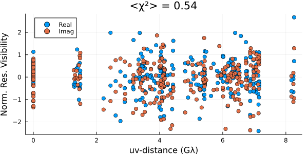
These look reasonable, although there may be some minor overfitting. This could be improved in a few ways, but that is beyond the goal of this quick tutorial. Plotting the image, we see that we have a much cleaner version of the closure-only image from Imaging a Black Hole using only Closure Quantities.
import CairoMakie as CM
g = imagepixels(fovx, fovy, 128, 128)
img = intensitymap(skymodel(post, xopt), g)
imageviz(img, size=(500, 400))|> DisplayAs.PNG |> DisplayAs.Text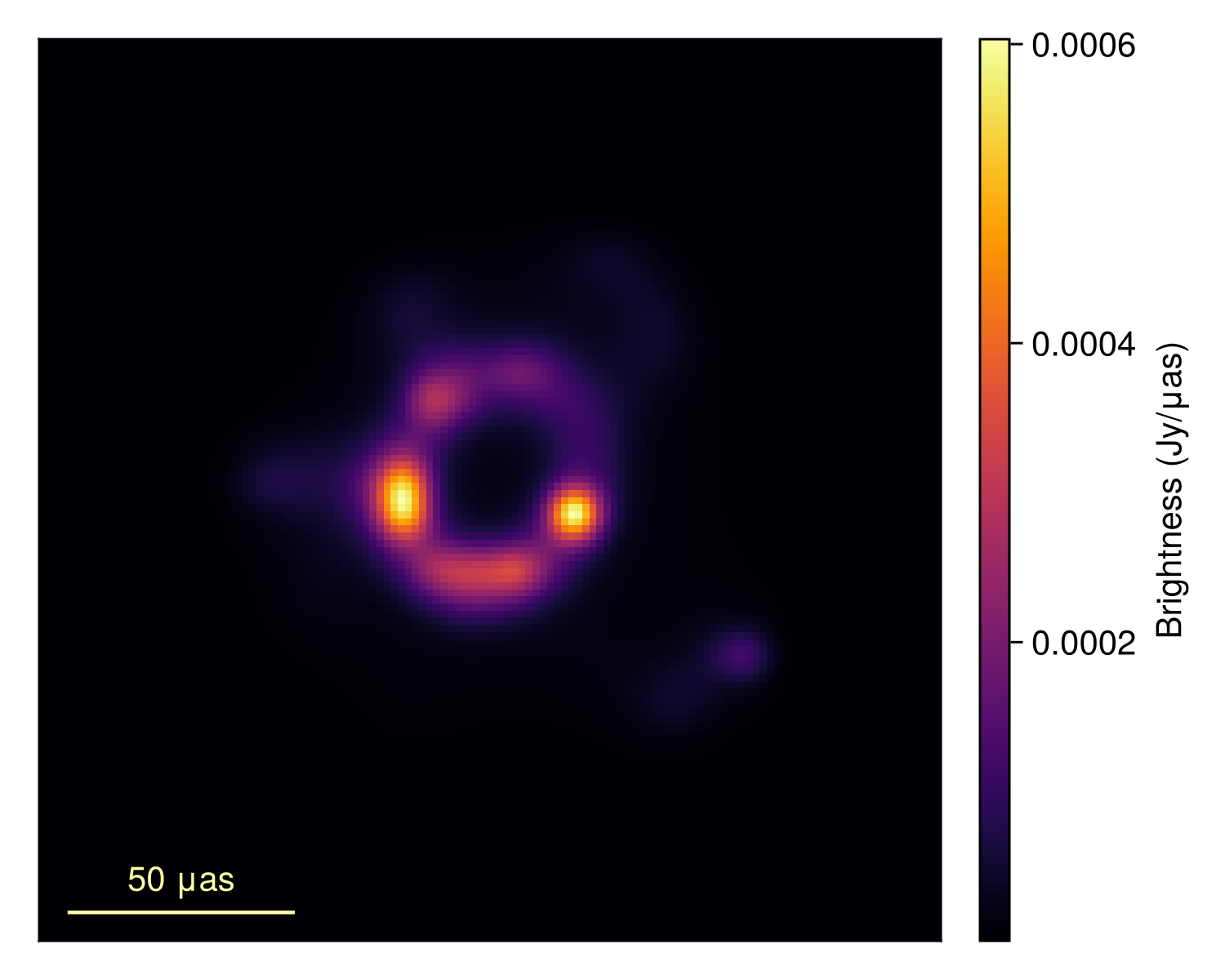
Because we also fit the instrument model, we can inspect their parameters. To do this, Comrade provides a caltable function that converts the flattened gain parameters to a tabular format based on the time and its segmentation.
intopt = instrumentmodel(post, xopt)
gt = Comrade.caltable(angle.(intopt))
plot(gt, layout=(3,3), size=(600,500)) |> DisplayAs.PNG |> DisplayAs.Text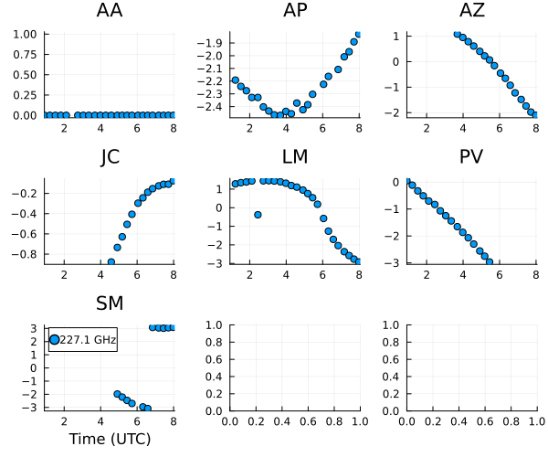
The gain phases are pretty random, although much of this is due to us picking a random reference sites for each scan.
Moving onto the gain amplitudes, we see that most of the gain variation is within 10% as expected except LMT, which has massive variations.
gt = Comrade.caltable(abs.(intopt))
plot(gt, layout=(3,3), size=(600,500)) |> DisplayAs.PNG |> DisplayAs.Text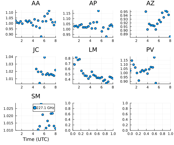
To sample from the posterior, we will use HMC, specifically the NUTS algorithm. For information about NUTS, see Michael Betancourt's notes. However, due to the need to sample a large number of gain parameters, constructing the posterior is rather time-consuming. Therefore, for this tutorial, we will only do a quick preliminary run
using AdvancedHMC
chain = sample(rng, post, NUTS(0.8), 1_000; n_adapts=500, progress=false, initial_params=xopt)
PosteriorSamples
Samples size: (1000,)
sampler used: AHMC
Mean
┌─────────────────────────────────────────────────────────────────────────────────────────────────────────────────────────────────────────────────────────────────────────────────────────────────────────────────────────────────────────────────────────────┬───────────────────────────────────────────────────────────────────────────────────────────────────────────────────────────────────────────────────────────────────────────────────────────────────────────────────────────────────────────────────────────────────────────────────────────────────────────────────────────────────────────────────────────────────────────────────────────────────────────────────────────────┐
│ sky │ instrument │
│ @NamedTuple{c::@NamedTuple{params::Matrix{Float64}, hyperparams::Float64}, σimg::Float64, fg::Float64} │ @NamedTuple{lg::Comrade.SiteArray{Float64, 1, Vector{Float64}, Vector{Comrade.IntegrationTime{Int64, Float64}}, Vector{Comrade.FrequencyChannel{Float64, Int64}}, Vector{Symbol}}, gp::Comrade.SiteArray{Float64, 1, Vector{Float64}, Vector{Comrade.IntegrationTime{Int64, Float64}}, Vector{Comrade.FrequencyChannel{Float64, Int64}}, Vector{Symbol}}} │
├─────────────────────────────────────────────────────────────────────────────────────────────────────────────────────────────────────────────────────────────────────────────────────────────────────────────────────────────────────────────────────────────┼───────────────────────────────────────────────────────────────────────────────────────────────────────────────────────────────────────────────────────────────────────────────────────────────────────────────────────────────────────────────────────────────────────────────────────────────────────────────────────────────────────────────────────────────────────────────────────────────────────────────────────────────┤
│ (c = (params = [0.0573276 0.0538736 … 0.00488822 -0.0172816; 0.0359576 0.0959193 … 0.0234177 0.0164586; … ; -0.0192619 0.0125053 … 0.0500033 0.0376541; -0.0249554 0.00524119 … 0.0192785 0.0142931], hyperparams = 25.0136), σimg = 2.12507, fg = 0.39382) │ (lg = [0.0150747, 0.0293885, 0.00742315, 0.0270556, -0.365148, 0.1374, 0.0040934, 0.0290342, -0.18744, 0.101348 … -0.071373, 0.01442, -0.87302, 0.0135293, 0.00643316, 0.0293774, -0.13733, 0.0209674, -0.920339, 0.0112785], gp = [0.0, -0.839375, 0.0, -2.19094, 0.929352, -1.00414, 0.0, -2.24147, 0.991197, -1.21789 … -2.35556, -0.10368, 0.566519, 0.890397, 0.0, -1.83052, -2.4496, -0.0706572, 1.78576, 0.58547]) │
└─────────────────────────────────────────────────────────────────────────────────────────────────────────────────────────────────────────────────────────────────────────────────────────────────────────────────────────────────────────────────────────────┴───────────────────────────────────────────────────────────────────────────────────────────────────────────────────────────────────────────────────────────────────────────────────────────────────────────────────────────────────────────────────────────────────────────────────────────────────────────────────────────────────────────────────────────────────────────────────────────────────────────────────────────────┘
Std. Dev.
┌──────────────────────────────────────────────────────────────────────────────────────────────────────────────────────────────────────────────────────────────────────────────────────────────────────────────────────────────────────────┬─────────────────────────────────────────────────────────────────────────────────────────────────────────────────────────────────────────────────────────────────────────────────────────────────────────────────────────────────────────────────────────────────────────────────────────────────────────────────────────────────────────────────────────────────────────────────────────────────────────────────────────────┐
│ sky │ instrument │
│ @NamedTuple{c::@NamedTuple{params::Matrix{Float64}, hyperparams::Float64}, σimg::Float64, fg::Float64} │ @NamedTuple{lg::Comrade.SiteArray{Float64, 1, Vector{Float64}, Vector{Comrade.IntegrationTime{Int64, Float64}}, Vector{Comrade.FrequencyChannel{Float64, Int64}}, Vector{Symbol}}, gp::Comrade.SiteArray{Float64, 1, Vector{Float64}, Vector{Comrade.IntegrationTime{Int64, Float64}}, Vector{Comrade.FrequencyChannel{Float64, Int64}}, Vector{Symbol}}} │
├──────────────────────────────────────────────────────────────────────────────────────────────────────────────────────────────────────────────────────────────────────────────────────────────────────────────────────────────────────────┼─────────────────────────────────────────────────────────────────────────────────────────────────────────────────────────────────────────────────────────────────────────────────────────────────────────────────────────────────────────────────────────────────────────────────────────────────────────────────────────────────────────────────────────────────────────────────────────────────────────────────────────────┤
│ (c = (params = [0.563501 0.589334 … 0.593533 0.539414; 0.556654 0.644251 … 0.666653 0.564394; … ; 0.574945 0.629623 … 0.680237 0.603878; 0.54545 0.594395 … 0.575289 0.536462], hyperparams = 14.4053), σimg = 0.230306, fg = 0.0473921) │ (lg = [0.162626, 0.158748, 0.0188518, 0.0207866, 0.074927, 0.0610893, 0.0180926, 0.0208276, 0.0662911, 0.0604902 … 0.0462921, 0.0187898, 0.0637396, 0.0171076, 0.017122, 0.0215309, 0.0484268, 0.018186, 0.0650645, 0.0173966], gp = [0.0, 0.541244, 0.0, 0.0177601, 0.225427, 0.546062, 0.0, 0.0175076, 0.226513, 0.55077 … 0.453412, 0.304571, 2.92437, 2.76177, 0.0, 0.01798, 0.595878, 0.302948, 2.29582, 2.84881]) │
└──────────────────────────────────────────────────────────────────────────────────────────────────────────────────────────────────────────────────────────────────────────────────────────────────────────────────────────────────────────┴─────────────────────────────────────────────────────────────────────────────────────────────────────────────────────────────────────────────────────────────────────────────────────────────────────────────────────────────────────────────────────────────────────────────────────────────────────────────────────────────────────────────────────────────────────────────────────────────────────────────────────────────┘Note
The above sampler will store the samples in memory, i.e. RAM. For large models this can lead to out-of-memory issues. To fix that you can include the keyword argument saveto = DiskStore() which periodically saves the samples to disk limiting memory useage. You can load the chain using load_samples(diskout) where diskout is the object returned from sample.
Now we prune the adaptation phase
chain = chain[501:end]PosteriorSamples
Samples size: (500,)
sampler used: AHMC
Mean
┌─────────────────────────────────────────────────────────────────────────────────────────────────────────────────────────────────────────────────────────────────────────────────────────────────────────────────────────────────────────────────────────────────┬───────────────────────────────────────────────────────────────────────────────────────────────────────────────────────────────────────────────────────────────────────────────────────────────────────────────────────────────────────────────────────────────────────────────────────────────────────────────────────────────────────────────────────────────────────────────────────────────────────────────────────────────────────┐
│ sky │ instrument │
│ @NamedTuple{c::@NamedTuple{params::Matrix{Float64}, hyperparams::Float64}, σimg::Float64, fg::Float64} │ @NamedTuple{lg::Comrade.SiteArray{Float64, 1, Vector{Float64}, Vector{Comrade.IntegrationTime{Int64, Float64}}, Vector{Comrade.FrequencyChannel{Float64, Int64}}, Vector{Symbol}}, gp::Comrade.SiteArray{Float64, 1, Vector{Float64}, Vector{Comrade.IntegrationTime{Int64, Float64}}, Vector{Comrade.FrequencyChannel{Float64, Int64}}, Vector{Symbol}}} │
├─────────────────────────────────────────────────────────────────────────────────────────────────────────────────────────────────────────────────────────────────────────────────────────────────────────────────────────────────────────────────────────────────┼───────────────────────────────────────────────────────────────────────────────────────────────────────────────────────────────────────────────────────────────────────────────────────────────────────────────────────────────────────────────────────────────────────────────────────────────────────────────────────────────────────────────────────────────────────────────────────────────────────────────────────────────────────┤
│ (c = (params = [0.0719643 0.0510149 … 0.00828992 -0.00271699; 0.0187249 0.0319039 … 0.0121522 -0.0100052; … ; -0.0591724 -0.0461885 … 0.0349365 0.0432505; -0.0270872 -0.0207295 … 0.0528356 0.0220332], hyperparams = 23.3533), σimg = 2.14631, fg = 0.393779) │ (lg = [0.014644, 0.0203603, 0.00682733, 0.0278125, -0.351699, 0.128658, 0.00575145, 0.0276147, -0.176857, 0.0931215 … -0.0740699, 0.0144409, -0.870298, 0.013699, 0.00628928, 0.0296579, -0.142519, 0.0202157, -0.915686, 0.0109718], gp = [0.0, -1.06469, 0.0, -2.19113, 0.854401, -1.23153, 0.0, -2.24061, 0.916516, -1.44655 … -2.40848, -0.0947116, 1.16288, 0.85511, 0.0, -1.83049, -2.47157, -0.060477, 2.14831, 0.533863]) │
└─────────────────────────────────────────────────────────────────────────────────────────────────────────────────────────────────────────────────────────────────────────────────────────────────────────────────────────────────────────────────────────────────┴───────────────────────────────────────────────────────────────────────────────────────────────────────────────────────────────────────────────────────────────────────────────────────────────────────────────────────────────────────────────────────────────────────────────────────────────────────────────────────────────────────────────────────────────────────────────────────────────────────────────────────────────────────┘
Std. Dev.
┌──────────────────────────────────────────────────────────────────────────────────────────────────────────────────────────────────────────────────────────────────────────────────────────────────────────────────────────────────────────┬────────────────────────────────────────────────────────────────────────────────────────────────────────────────────────────────────────────────────────────────────────────────────────────────────────────────────────────────────────────────────────────────────────────────────────────────────────────────────────────────────────────────────────────────────────────────────────────────────────────────────────────────┐
│ sky │ instrument │
│ @NamedTuple{c::@NamedTuple{params::Matrix{Float64}, hyperparams::Float64}, σimg::Float64, fg::Float64} │ @NamedTuple{lg::Comrade.SiteArray{Float64, 1, Vector{Float64}, Vector{Comrade.IntegrationTime{Int64, Float64}}, Vector{Comrade.FrequencyChannel{Float64, Int64}}, Vector{Symbol}}, gp::Comrade.SiteArray{Float64, 1, Vector{Float64}, Vector{Comrade.IntegrationTime{Int64, Float64}}, Vector{Comrade.FrequencyChannel{Float64, Int64}}, Vector{Symbol}}} │
├──────────────────────────────────────────────────────────────────────────────────────────────────────────────────────────────────────────────────────────────────────────────────────────────────────────────────────────────────────────┼────────────────────────────────────────────────────────────────────────────────────────────────────────────────────────────────────────────────────────────────────────────────────────────────────────────────────────────────────────────────────────────────────────────────────────────────────────────────────────────────────────────────────────────────────────────────────────────────────────────────────────────────┤
│ (c = (params = [0.559622 0.593387 … 0.609726 0.499302; 0.563461 0.641451 … 0.697687 0.594632; … ; 0.568903 0.630401 … 0.67006 0.597145; 0.545704 0.609378 … 0.596218 0.528706], hyperparams = 14.0067), σimg = 0.237173, fg = 0.0500717) │ (lg = [0.158259, 0.1544, 0.0188616, 0.0209098, 0.0698608, 0.0603248, 0.0188366, 0.0211576, 0.0592879, 0.0595879 … 0.0443811, 0.0186425, 0.0562753, 0.0170632, 0.0179296, 0.0215981, 0.0467794, 0.0190166, 0.0570355, 0.0179949], gp = [0.0, 0.447546, 0.0, 0.0178055, 0.218704, 0.451569, 0.0, 0.0176554, 0.219952, 0.45331 … 0.592607, 0.346311, 2.72841, 2.75389, 0.0, 0.0179481, 0.809581, 0.339932, 1.90362, 2.84272]) │
└──────────────────────────────────────────────────────────────────────────────────────────────────────────────────────────────────────────────────────────────────────────────────────────────────────────────────────────────────────────┴────────────────────────────────────────────────────────────────────────────────────────────────────────────────────────────────────────────────────────────────────────────────────────────────────────────────────────────────────────────────────────────────────────────────────────────────────────────────────────────────────────────────────────────────────────────────────────────────────────────────────────────────┘Warning
This should be run for likely an order of magnitude more steps to properly estimate expectations of the posterior
Now that we have our posterior, we can put error bars on all of our plots above. Let's start by finding the mean and standard deviation of the gain phases
mchain = Comrade.rmap(mean, chain);
schain = Comrade.rmap(std, chain);
Now we can use the measurements package to automatically plot everything with error bars. First we create a caltable the same way but making sure all of our variables have errors attached to them.
using Measurements
gmeas = instrumentmodel(post, (;instrument= map((x,y)->Measurements.measurement.(x,y), mchain.instrument, schain.instrument)))
ctable_am = caltable(abs.(gmeas))
ctable_ph = caltable(angle.(gmeas))
─────────┬───────────────────┬────────────────────────────────────────────────────────────────────────────────────
Ti │ Fr │ AA AP AZ JC LM PV SM
─────────┼───────────────────┼────────────────────────────────────────────────────────────────────────────────────
0.92 hr │ 227.070703125 GHz │ 0.0±0.0 missing missing missing missing -1.06±0.45 missing
1.22 hr │ 227.070703125 GHz │ 0.0±0.0 -2.191±0.018 missing missing 0.85±0.22 -1.23±0.45 missing
1.52 hr │ 227.070703125 GHz │ 0.0±0.0 -2.241±0.018 missing missing 0.92±0.22 -1.45±0.45 missing
1.82 hr │ 227.070703125 GHz │ 0.0±0.0 -2.275±0.018 missing missing 0.95±0.22 -1.64±0.46 missing
2.12 hr │ 227.070703125 GHz │ 0.0±0.0 -2.328±0.018 missing missing 1.01±0.22 -1.83±0.46 missing
2.45 hr │ 227.070703125 GHz │ missing -2.328±0.018 missing missing -0.81±0.23 -1.9±0.71 missing
2.75 hr │ 227.070703125 GHz │ 0.0±0.0 -2.403±0.019 missing missing 1.01±0.23 -2.01±0.99 missing
3.05 hr │ 227.070703125 GHz │ 0.0±0.0 -2.435±0.019 missing missing 1.01±0.23 -2.1±1.2 missing
3.35 hr │ 227.070703125 GHz │ 0.0±0.0 -2.464±0.018 missing missing 0.99±0.24 -1.9±1.7 missing
3.68 hr │ 227.070703125 GHz │ 0.0±0.0 -2.469±0.017 0.61±0.25 missing 0.95±0.24 -1.4±2.3 missing
3.98 hr │ 227.070703125 GHz │ 0.0±0.0 -2.437±0.02 0.48±0.26 missing 0.88±0.24 -0.37±2.8 missing
4.28 hr │ 227.070703125 GHz │ 0.0±0.0 -2.457±0.019 0.31±0.26 missing 0.76±0.24 0.62±2.7 missing
4.58 hr │ 227.070703125 GHz │ 0.0±0.0 -2.371±0.019 0.14±0.27 -1.17±0.31 0.67±0.24 1.3±2.4 missing
4.92 hr │ 227.070703125 GHz │ 0.0±0.0 -2.424±0.02 -0.07±0.27 -0.99±0.32 0.52±0.25 1.9±1.7 -2.16±0.64
5.18 hr │ 227.070703125 GHz │ 0.0±0.0 -2.384±0.017 -0.25±0.27 -0.86±0.34 0.32±0.25 2.0±1.3 -2.28±0.9
5.45 hr │ 227.070703125 GHz │ 0.0±0.0 -2.303±0.019 -0.41±0.27 -0.71±0.34 0.1±0.25 2.05±0.87 -2.2±1.4
5.72 hr │ 227.070703125 GHz │ 0.0±0.0 missing -0.63±0.27 -0.58±0.35 -0.25±0.25 missing -1.8±2.2
6.05 hr │ 227.070703125 GHz │ 0.0±0.0 -2.224±0.02 -0.93±0.27 -0.43±0.36 -1.01±0.25 missing missing
6.32 hr │ 227.070703125 GHz │ 0.0±0.0 -2.163±0.018 -1.13±0.27 -0.35±0.36 -1.7±0.24 missing -0.35±2.9
6.58 hr │ 227.070703125 GHz │ 0.0±0.0 missing -1.41±0.27 -0.26±0.36 -2.14±0.24 missing 0.31±2.9
6.85 hr │ 227.070703125 GHz │ 0.0±0.0 -2.109±0.019 -1.71±0.27 -0.2±0.36 -2.43±0.54 missing 0.96±2.7
7.18 hr │ 227.070703125 GHz │ 0.0±0.0 -2.009±0.018 -1.97±0.26 -0.14±0.36 -2.3±1.6 missing 1.0±2.7
7.45 hr │ 227.070703125 GHz │ 0.0±0.0 -1.969±0.018 -2.22±0.35 -0.1±0.35 -1.3±2.6 missing 1.1±2.6
7.72 hr │ 227.070703125 GHz │ 0.0±0.0 -1.892±0.018 -2.41±0.59 -0.095±0.35 1.2±2.7 missing 0.86±2.8
7.98 hr │ 227.070703125 GHz │ 0.0±0.0 -1.83±0.018 -2.47±0.81 -0.06±0.34 2.1±1.9 missing 0.53±2.8
─────────┴───────────────────┴────────────────────────────────────────────────────────────────────────────────────Now let's plot the phase curves
plot(ctable_ph, layout=(4,3), size=(600,500)) |> DisplayAs.PNG |> DisplayAs.Text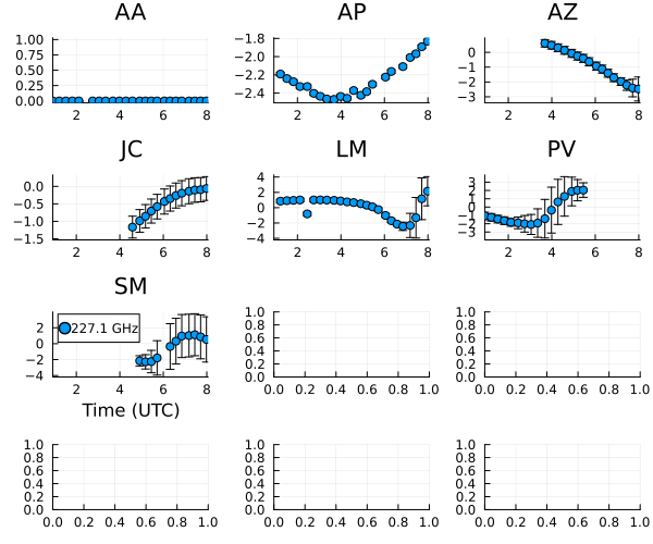
and now the amplitude curves
plot(ctable_am, layout=(4,3), size=(600,500)) |> DisplayAs.PNG |> DisplayAs.Text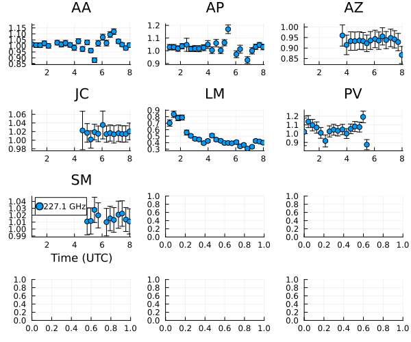
Finally let's construct some representative image reconstructions.
samples = skymodel.(Ref(post), chain[begin:5:end])
imgs = intensitymap.(samples, Ref(g))

mimg = mean(imgs)
simg = std(imgs)
fig = CM.Figure(;resolution=(700, 700));
axs = [CM.Axis(fig[i, j], xreversed=true, aspect=1) for i in 1:2, j in 1:2]
CM.image!(axs[1,1], mimg, colormap=:afmhot); axs[1, 1].title="Mean"
CM.image!(axs[1,2], simg./(max.(mimg, 1e-8)), colorrange=(0.0, 2.0), colormap=:afmhot);axs[1,2].title = "Std"
CM.image!(axs[2,1], imgs[1],   colormap=:afmhot);
CM.image!(axs[2,2], imgs[end], colormap=:afmhot);
CM.hidedecorations!.(axs)
fig |> DisplayAs.PNG |> DisplayAs.Text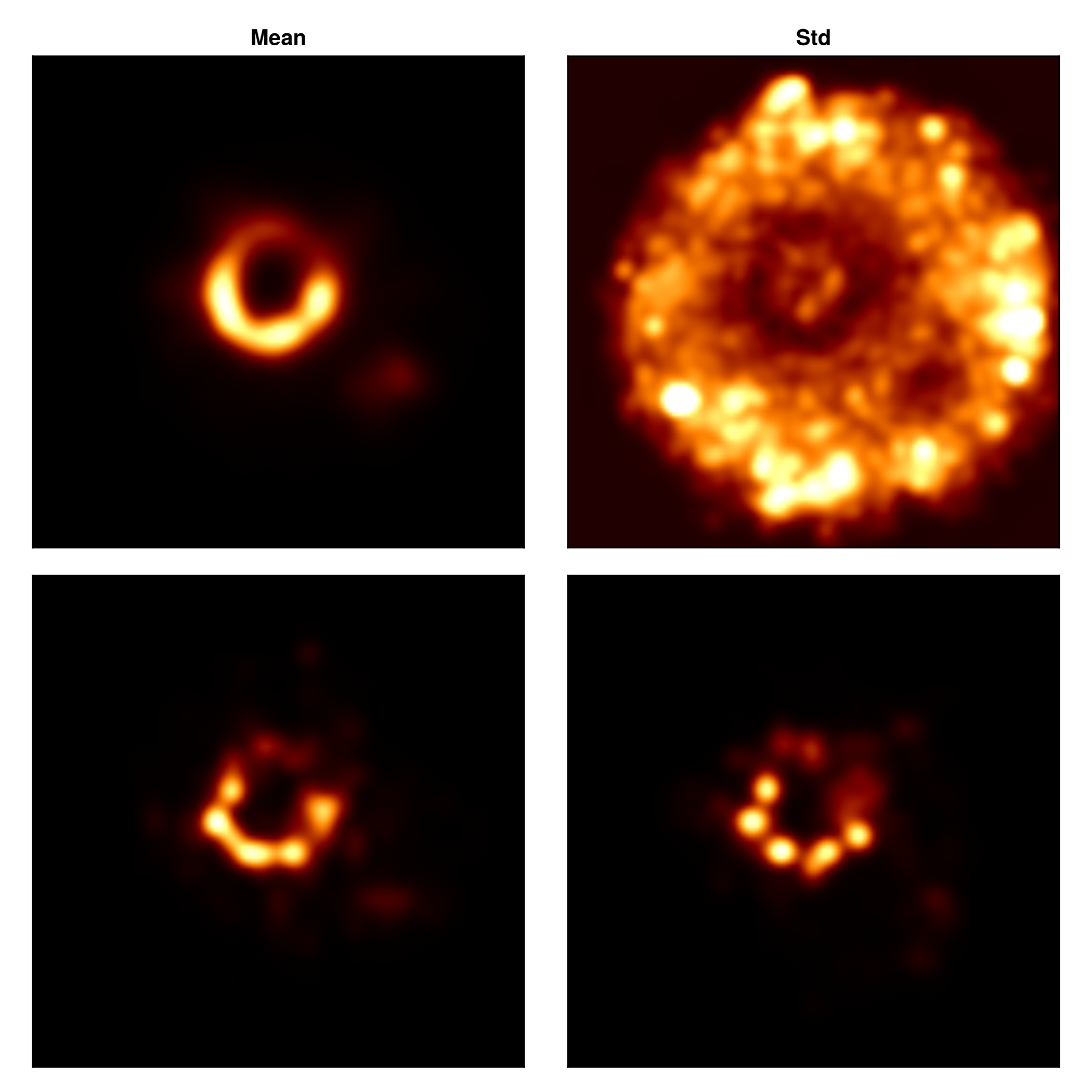
And viola, you have just finished making a preliminary image and instrument model reconstruction. In reality, you should run the sample step for many more MCMC steps to get a reliable estimate for the reconstructed image and instrument model parameters.
This page was generated using Literate.jl.