Hybrid Imaging of a Black Hole

In this tutorial, we will use hybrid imaging to analyze the 2017 EHT data. By hybrid imaging, we mean decomposing the model into simple geometric models, e.g., rings and such, plus a rasterized image model to soak up the additional structure. This approach was first developed in BB20 and applied to EHT 2017 data. We will use a similar model in this tutorial.

Introduction to Hybrid modeling and imaging

The benefit of using a hybrid-based modeling approach is the effective compression of information/parameters when fitting the data. Hybrid modeling requires the user to incorporate specific knowledge of how you expect the source to look like. For instance for M87, we expect the image to be dominated by a ring-like structure. Therefore, instead of using a high-dimensional raster to recover the ring, we can use a ring model plus a raster to soak up the additional degrees of freedom. This is the approach we will take in this tutorial to analyze the April 6 2017 EHT data of M87.

"nul"

Loading the Data

To get started we will load Comrade

using Comrade

Load the Data

using Pyehtim

For reproducibility we use a stable random number genreator

using StableRNGs
rng = StableRNG(42)

StableRNGs.LehmerRNG(state=0x00000000000000000000000000000055)

To download the data visit https://doi.org/10.25739/g85n-f134 To load the eht-imaging obsdata object we do:

obs = ehtim.obsdata.load_uvfits(joinpath(__DIR, "..", "..", "Data", "SR1_M87_2017_096_lo_hops_netcal_StokesI.uvfits"))

Python: <ehtim.obsdata.Obsdata object at 0x7f55dd2a7e20>

Now we do some minor preprocessing:

• Scan average the data since the data have been preprocessed so that the gain phases coherent.

obs = scan_average(obs).add_fractional_noise(0.02)

Python: <ehtim.obsdata.Obsdata object at 0x7f55bf235390>

For this tutorial we will once again fit complex visibilities since they provide the most information once the telescope/instrument model are taken into account.

dvis  = extract_table(obs, Visibilities())

EHTObservationTable{Comrade.EHTVisibilityDatum{:I}}
  source:      M87
  mjd:         57849
  bandwidth:   1.856e9
  sites:       [:AA, :AP, :AZ, :JC, :LM, :PV, :SM]
  nsamples:    274

Building the Model/Posterior

Now we build our intensity/visibility model. That is, the model that takes in a named tuple of parameters and perhaps some metadata required to construct the model. For our model, we will use a raster or ContinuousImage model, an m-ring model, and a large asymmetric Gaussian component to model the unresolved short-baseline flux.

function sky(θ, metadata)
    (;c, σimg, f, r, σ, τ, ξτ, ma, mp, fg) = θ
    (;ftot, grid) = metadata
    # Form the image model
    # First transform to simplex space first applying the non-centered transform
    rast = (ftot*f*(1-fg)).*to_simplex(CenteredLR(), σimg.*c)
    mimg = ContinuousImage(rast, grid, BSplinePulse{3}())
    # Form the ring model
    α = ma.*cos.(mp .- ξτ)
    β = ma.*sin.(mp .- ξτ)
    ring = smoothed(modify(MRing(α, β), Stretch(r, r*(1+τ)), Rotate(ξτ), Renormalize((ftot*(1-f)*(1-fg)))), σ)
    gauss = modify(Gaussian(), Stretch(μas2rad(250.0)), Renormalize(ftot*f*fg))
    # We group the geometric models together for improved efficiency. This will be
    # automated in future versions.
    return mimg + (ring + gauss)
end

sky (generic function with 1 method)

Unlike other imaging examples (e.g., Imaging a Black Hole using only Closure Quantities) we also need to include a model for the instrument, i.e., gains as well. The gains will be broken into two components

• Gain amplitudes which are typically known to 10-20%, except for LMT, which has amplitudes closer to 50-100%.

• Gain phases which are more difficult to constrain and can shift rapidly.

using VLBIImagePriors
using Distributions, DistributionsAD
G = SingleStokesGain() do x
    lg = x.lg
    gp = x.gp
    return exp(lg + 1im*gp)
end

intpr = (
    lg= ArrayPrior(IIDSitePrior(ScanSeg(), Normal(0.0, 0.2)); LM = IIDSitePrior(ScanSeg(), Normal(0.0, 1.0))),
    gp= ArrayPrior(IIDSitePrior(ScanSeg(), DiagonalVonMises(0.0, inv(π^2))); refant=SEFDReference(0.0))
        )
intmodel = InstrumentModel(G, intpr)

InstrumentModel
  with Jones:  SingleStokesGain
  with reference basis: CirBasis()

Before we move on, let's go into the model function a bit. This function takes two arguments θ and metadata. The θ argument is a named tuple of parameters that are fit to the data. The metadata argument is all the ancillary information we need to construct the model. For our hybrid model, we will need two variables for the metadata, a grid that specifies the locations of the image pixels and a cache that defines the algorithm used to calculate the visibilities given the image model. This is required since ContinuousImage is most easily computed using number Fourier transforms like the NFFT or FFT. To combine the models, we use Comrade's overloaded + operators, which will combine the images such that their intensities and visibilities are added pointwise.

Now let's define our metadata. First we will define the cache for the image. This is required to compute the numerical Fourier transform.

fovxy  = μas2rad(200.0)
npix   = 32
g      = imagepixels(fovxy, fovxy, npix, npix)

RectiGrid(
executor: Serial()
Dimensions: 
↓ X Sampled{Float64} LinRange{Float64}(-4.69663253574863e-10, 4.69663253574863e-10, 32) ForwardOrdered Regular Points,
→ Y Sampled{Float64} LinRange{Float64}(-4.69663253574863e-10, 4.69663253574863e-10, 32) ForwardOrdered Regular Points
)

Part of hybrid imaging is to force a scale separation between the different model components to make them identifiable. To enforce this we will set the length scale of the raster component equal to the beam size of the telescope in units of pixel length, which is given by

beam = beamsize(dvis)
rat = (beam/(step(g.X)))
cprior = GaussMarkovRandomField(rat, size(g); order=2)

GaussMarkovRandomField(
Graph: MarkovRandomFieldGraph{2}(
dims: (32, 32)
)
Correlation Parameter: 3.9947524783031394
)

additionlly we will fix the standard deviation of the field to unity and instead use a pseudo non-centered parameterization for the field. GaussMarkovRandomField(meanpr, 0.1*rat, 1.0, crcache)

Finally we can put form the total model prior

skyprior = (
          c  = cprior,
          σimg = truncated(Normal(0.0, 1.0); lower=0.01),
          f  = Uniform(0.0, 1.0),
          r  = Uniform(μas2rad(10.0), μas2rad(30.0)),
          σ  = Uniform(μas2rad(0.1), μas2rad(10.0)),
          τ  = truncated(Normal(0.0, 0.1); lower=0.0, upper=1.0),
          ξτ = Uniform(-π/2, π/2),
          ma = ntuple(_->Uniform(0.0, 0.5), 2),
          mp = ntuple(_->Uniform(0.0, 2π), 2),
          fg = Uniform(0.0, 1.0),
        )

(c = GaussMarkovRandomField(
Graph: MarkovRandomFieldGraph{2}(
dims: (32, 32)
)
Correlation Parameter: 3.9947524783031394
), σimg = Truncated(Distributions.Normal{Float64}(μ=0.0, σ=1.0); lower=0.01), f = Distributions.Uniform{Float64}(a=0.0, b=1.0), r = Distributions.Uniform{Float64}(a=4.84813681109536e-11, b=1.454441043328608e-10), σ = Distributions.Uniform{Float64}(a=4.848136811095359e-13, b=4.84813681109536e-11), τ = Truncated(Distributions.Normal{Float64}(μ=0.0, σ=0.1); lower=0.0, upper=1.0), ξτ = Distributions.Uniform{Float64}(a=-1.5707963267948966, b=1.5707963267948966), ma = (Distributions.Uniform{Float64}(a=0.0, b=0.5), Distributions.Uniform{Float64}(a=0.0, b=0.5)), mp = (Distributions.Uniform{Float64}(a=0.0, b=6.283185307179586), Distributions.Uniform{Float64}(a=0.0, b=6.283185307179586)), fg = Distributions.Uniform{Float64}(a=0.0, b=1.0))

Now we form the metadata

skymetadata = (;ftot=1.1, grid = g)
skym = SkyModel(sky, skyprior, g; metadata=skymetadata)

 SkyModel
  with map: sky
   on grid: RectiGrid

This is everything we need to specify our posterior distribution, which our is the main object of interest in image reconstructions when using Bayesian inference.

post = VLBIPosterior(skym, intmodel, dvis)

VLBIPosterior
ObservedSkyModel
  with map: sky
   on grid: FourierDualDomainObservedInstrumentModel
  with Jones:  SingleStokesGain
  with reference basis: CirBasis()Data Products: Comrade.EHTVisibilityDatum

To sample from our prior we can do

xrand = prior_sample(rng, post)

(sky = (c = [-2.1962796581148964 -1.1243036995667173 … 0.1809752675358745 0.5228771323078414; -0.3425595294889296 0.875841911517527 … -1.7473734958334282 -0.04613166448214303; … ; -1.0346864752090177 -0.3318267589886823 … 1.8169964745030398 0.9883988762644694; -0.17570171401278734 -1.1226297884080063 … 0.23776676295262178 -0.12297534720788651], σimg = 0.42179682054864803, f = 0.5609945096442908, r = 6.822575941314203e-11, σ = 1.3552947886307434e-11, τ = 0.06730160453188876, ξτ = -1.4000761734573677, ma = (0.34647334815942743, 0.2990582529227658), mp = (4.539841547826114, 0.12993729152293854), fg = 0.37817042117774347), instrument = (lg = [-0.05442203326486966, -0.06854489109756777, -0.03494199200648159, 0.01466628222962606, -0.5344934234689837, 0.06909851514694904, 0.16895161284675558, -0.35730974364294593, 2.2297802017289468, 0.14330481934854625  …  -0.2562770339996219, -0.13260692566162727, -0.3754572129527364, 0.13202624897901952, -0.22070992008362902, -0.14044807385292715, 0.08434814836495083, -0.16645257431733257, 0.07930960115946253, 0.09730314408987739], gp = [0.0, 0.801726817174358, 0.0, 0.5352791204380771, 1.2147806619090493, 1.8380953555627066, 0.0, -1.2091566463464445, 0.4316140924972767, 2.8356106901992013  …  0.6797921035265353, 1.5869294029613246, 1.9179548979911933, -0.7937725614627756, 0.0, -2.1551512461478652, -1.4071803931922073, -0.3657978469609746, -2.891016934890005, -1.059347481121196]))

and then plot the results

import CairoMakie as CM
gpl = imagepixels(μas2rad(200.0), μas2rad(200.0), 128, 128)
fig = imageviz(intensitymap(skymodel(post, xrand), gpl));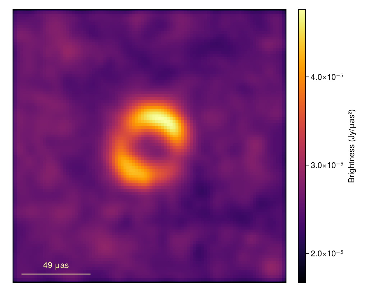

Reconstructing the Image

To find the image we will demonstrate two methods:

• Optimization to find the MAP (fast but often a poor estimator)

• Sampling to find the posterior (slow but provides a substantially better estimator)

For optimization we will use the Optimization.jl package and the LBFGS optimizer. To use this we use the comrade_opt function

using Optimization
using OptimizationOptimJL
using Zygote
xopt, sol = comrade_opt(post, LBFGS(), Optimization.AutoZygote(); initial_params=prior_sample(rng, post), maxiters=1000, g_tol=1e0)

((sky = (c = [-0.0995306744786591 -0.09436406938985524 … -0.18525562964756473 -0.030337828903544438; -0.0959182357878746 -0.11596729179467957 … -0.37157879207784805 -0.17478776939841134; … ; 0.15642345627105278 0.1625628038817072 … -0.008878853050988615 -0.02611953009792284; 0.14327090610592508 0.14283013815960469 … 0.0661996206475343 0.003967767890060875], σimg = 2.933987812457762, f = 0.7463644610433627, r = 1.0127176289055832e-10, σ = 1.3306586076675141e-11, τ = 0.10567360119399186, ξτ = -0.5950990085162118, ma = (0.2237020624892037, 0.12922801465964473), mp = (2.6796351307612687, 1.9988106309963085), fg = 0.09173697808174733), instrument = (lg = [-0.012159559838363707, -0.009110919263453717, 0.022943634711006595, 0.03755024273676404, -0.25154340299453615, 0.06411906964565808, 0.0149361883115565, 0.04166198846778192, 0.010107728287926832, 0.04465433950181079  …  0.0602553708530045, 0.0266051708002914, -0.35936755412679566, 0.025003825846650903, 0.02648729820107359, 0.03676120025984552, 0.045904092473444034, 0.033542243163054646, -0.4408318675037615, 0.02391952313446484], gp = [0.0, 0.2006412698814161, 0.0, -2.191452360318147, 1.4874356321254911, 0.046612615055883475, 0.0, -2.2413214519483087, 1.5395540073439222, -0.15112687766530053  …  -1.6896642237245887, 0.22240825837848313, -2.9633334987736557, -2.899523352483803, 0.0, -1.8298972632359474, -1.7718381019889156, 0.16771843348672513, -3.098952679865772, -2.9569638178372024])), retcode: Failure
u: [-0.0995306744786591, -0.0959182357878746, 0.06603011131757293, 0.2676411450121133, 0.20379782924247583, -0.0017579875089126428, -0.10532927264257444, -0.1131184842421163, -0.06519575768966857, -0.0548955992764885  …  -0.9078891143799345, -0.24064425671727102, -0.9192452955810075, -0.18733745541816227, 0.15656506638894255, 0.9247300480961397, -0.04007052639378467, -0.9391712746933522, -0.1721669155179959, -0.9218830335808508]
Final objective value:     -1526.7000375658124
)

First we will evaluate our fit by plotting the residuals

using Plots
fig = residual(post, xopt);

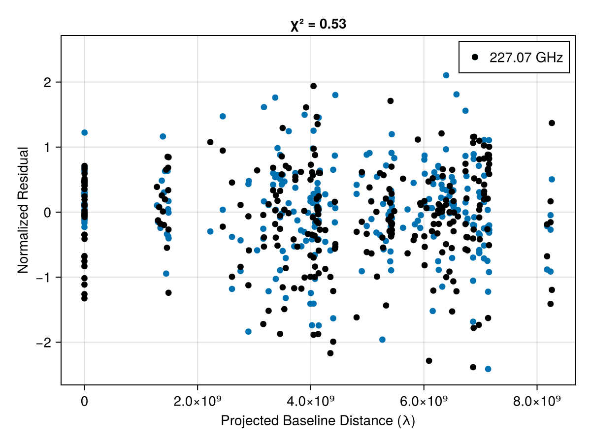
These residuals suggest that we are substantially overfitting the data. This is a common side effect of MAP imaging. As a result if we plot the image we see that there is substantial high-frequency structure in the image that isn't supported by the data.

imageviz(intensitymap(skymodel(post, xopt), gpl), figure=(;resolution=(500, 400),))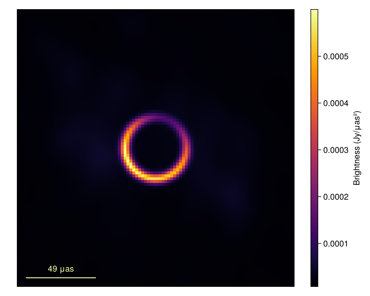

To improve our results we will now move to Posterior sampling. This is the main method we recommend for all inference problems in Comrade. While it is slower the results are often substantially better. To sample we will use the AdvancedHMC package.

using AdvancedHMC
chain = sample(rng, post, NUTS(0.8), 700; n_adapts=500, progress=false, initial_params=xopt);

[ Info: Found initial step size 0.0015625

We then remove the adaptation/warmup phase from our chain

chain = chain[501:end]

PosteriorSamples
  Samples size: (200,)
  sampler used: AHMC
Mean
┌───────────────────────────────────────────────────────────────────────────────
│ sky                                                                          ⋯
│ @NamedTuple{c::Matrix{Float64}, σimg::Float64, f::Float64, r::Float64, σ::Fl ⋯
├───────────────────────────────────────────────────────────────────────────────
│ (c = [-0.0931009 -0.187723 … -0.397124 -0.299192; -0.211345 -0.388092 … -0.5 ⋯
└───────────────────────────────────────────────────────────────────────────────
                                                               2 columns omitted
Std. Dev.
┌───────────────────────────────────────────────────────────────────────────────
│ sky                                                                          ⋯
│ @NamedTuple{c::Matrix{Float64}, σimg::Float64, f::Float64, r::Float64, σ::Fl ⋯
├───────────────────────────────────────────────────────────────────────────────
│ (c = [0.645031 0.702573 … 0.654324 0.608351; 0.720454 0.830057 … 0.761381 0. ⋯
└───────────────────────────────────────────────────────────────────────────────
                                                               2 columns omitted

Warning

This should be run for 4-5x more steps to properly estimate expectations of the posterior

Now lets plot the mean image and standard deviation images. To do this we first clip the first 250 MCMC steps since that is during tuning and so the posterior is not sampling from the correct sitesary distribution.

using StatsBase
msamples = skymodel.(Ref(post), chain[begin:2:end]);

The mean image is then given by

imgs = intensitymap.(msamples, Ref(gpl))
fig = imageviz(mean(imgs), colormap=:afmhot, size=(400, 300));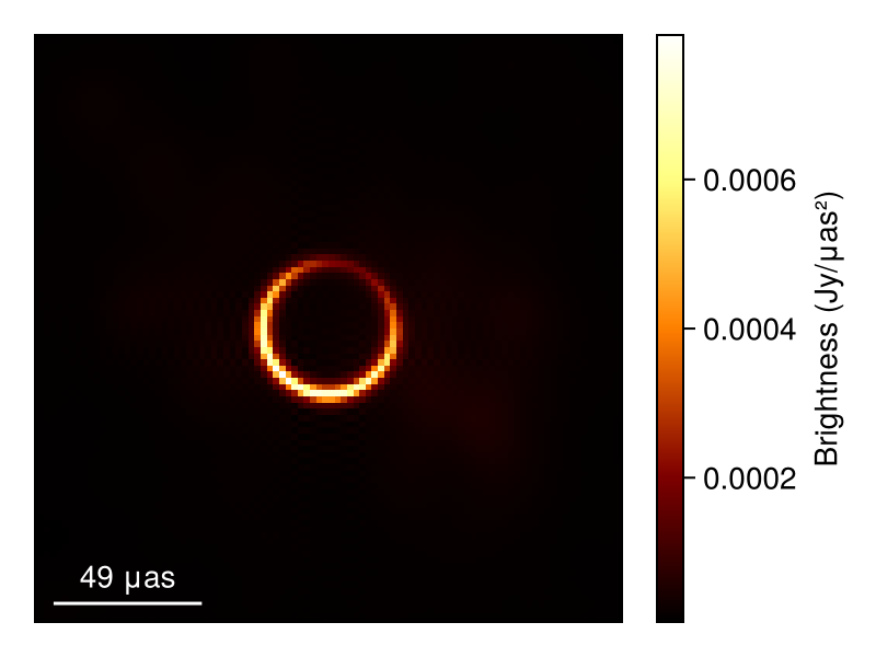

fig = imageviz(std(imgs), colormap=:batlow, size=(400, 300));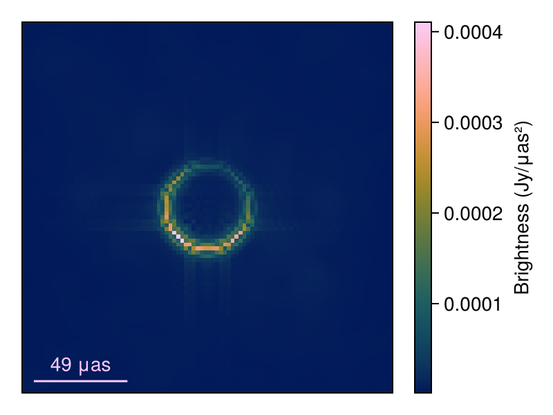

We can also split up the model into its components and analyze each separately

comp = Comrade.components.(msamples)
ring_samples = getindex.(comp, 2)
rast_samples = first.(comp)
ring_imgs = intensitymap.(ring_samples, Ref(gpl));
rast_imgs = intensitymap.(rast_samples, Ref(gpl));

ring_mean, ring_std = mean_and_std(ring_imgs);
rast_mean, rast_std = mean_and_std(rast_imgs);

fig = CM.Figure(; resolution=(400, 400));
axes = [CM.Axis(fig[i, j], xreversed=true, aspect=CM.DataAspect()) for i in 1:2, j in 1:2]
CM.image!(axes[1,1], ring_mean, colormap=:afmhot); axes[1,1].title = "Ring Mean"
CM.image!(axes[1,2], ring_std, colormap=:afmhot); axes[1,2].title = "Ring Std. Dev."
CM.image!(axes[2,1], rast_mean, colormap=:afmhot); axes[2,1].title = "Rast Mean"
CM.image!(axes[2,2], rast_std./rast_mean, colormap=:afmhot); axes[2,2].title = "Rast std/mean"
CM.hidedecorations!.(axes)
fig |> DisplayAs.PNG |> DisplayAs.Text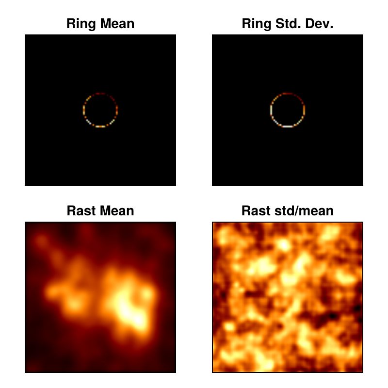

Finally, let's take a look at some of the ring parameters

figd = CM.Figure(;resolution=(650, 400));
p1 = CM.density(figd[1,1], rad2μas(chain.sky.r)*2, axis=(xlabel="Ring Diameter (μas)",))
p2 = CM.density(figd[1,2], rad2μas(chain.sky.σ)*2*sqrt(2*log(2)), axis=(xlabel="Ring FWHM (μas)",))
p3 = CM.density(figd[1,3], -rad2deg.(chain.sky.mp.:1) .+ 360.0, axis=(xlabel = "Ring PA (deg) E of N",))
p4 = CM.density(figd[2,1], 2*chain.sky.ma.:2, axis=(xlabel="Brightness asymmetry",))
p5 = CM.density(figd[2,2], 1 .- chain.sky.f, axis=(xlabel="Ring flux fraction",))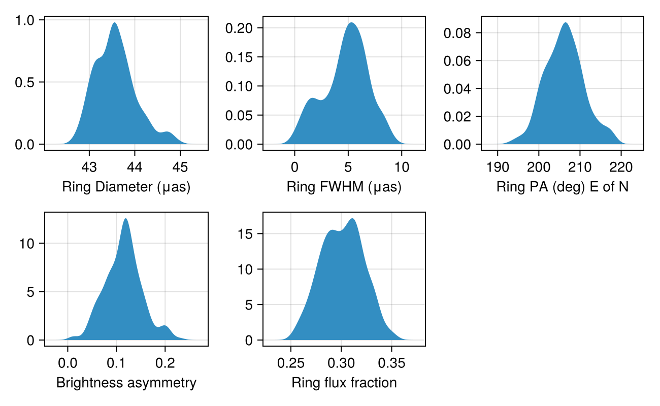

Now let's check the residuals using draws from the posterior

p = Plots.plot();
for s in sample(chain, 10)
    residual!(p, post, s, legend=false)
end

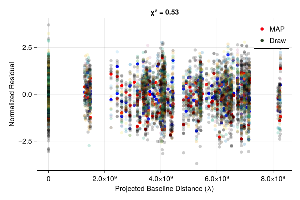
And everything looks pretty good! Now comes the hard part: interpreting the results...

---

This page was generated using Literate.jl.