Polarized Image and Instrumental Modeling

In this tutorial, we will analyze a simulated simple polarized dataset to demonstrate Comrade's polarized imaging capabilities.

Introduction to Polarized Imaging

The EHT is a polarized interferometer. However, like all VLBI interferometers, it does not directly measure the Stokes parameters (I, Q, U, V). Instead, it measures components related to the electric field at the telescope along two directions using feeds. There are two types of feeds at telescopes: circular, which measure $R / L$ components of the electric field, and linear feeds, which measure $X / Y$ components of the electric field. Most sites in the EHT use circular feeds, meaning they measure the right (R) and left electric field (L) at each telescope. Although note that ALMA actually uses linear feeds. Currently Comrade has the ability to fit natively mixed polarization data however, the publically released EHT data has been converted to circular polarization. For a VLBI array whose feeds are purely circluar the coherency matrices are given by,

C_{i j} = (\begin{matrix} R R^{*} & R L^{*} \\ L R^{*} & L L^{*} \end{matrix}) .

These coherency matrices are the fundamental object in interferometry and what the telescope observes. For a perfect interferometer, these circular coherency matrices are related to the usual Fourier transform of the stokes parameters by

(\begin{matrix} \tilde{I} \\ \tilde{Q} \\ \tilde{U} \\ \tilde{V} \end{matrix}) = \frac{1}{2} (\begin{matrix} R R^{*} + L L^{*} \\ R L^{*} + L R^{*} \\ i (L R^{*} - R L^{*}) \\ R R^{*} - L L^{*} \end{matrix}) .

Note

In this tutorial, we stick to circular feeds but Comrade has the capabilities to model linear (XX,XY, ...) and mixed basis coherencies (e.g., RX, RY, ...).

In reality, the measure coherencies are corrupted by both the atmosphere and the telescope itself. In Comrade we use the RIME formalism ^[1] to represent these corruptions, namely our measured coherency matrices $V_{i j}$ are given by

V_{i j} = J_{i} C_{i j} J_{j}^{†}

where $J$ is known as a Jones matrix and $i j$ denotes the baseline $i j$ with sites $i$ and $j$ .

Comrade is highly flexible with how the Jones matrices are formed and provides several convenience functions that parameterize standard Jones matrices. These matrices include:

JonesG which builds the set of complex gain Jones matrices

G = (\begin{matrix} g_{a} & 0 \\ 0 & g_{b} \end{matrix})

JonesD which builds the set of complex d-terms Jones matrices

D = (\begin{matrix} 1 & d_{a} \\ d_{b} & 1 \end{matrix})

JonesR is the ideal telescope response $R$ . This transformation is special and combines two things using the decomposition $R = F B$ . The first, $B$ , is the transformation from some reference basis to the observed coherency basis (this allows for mixed basis measurements). The second is the feed rotation, $F$ , that transforms from some reference axis to the axis of the telescope as the source moves in the sky. The feed rotation matrix F for circular feeds in terms of the per station feed rotation angle $φ$ is

F = (\begin{matrix} e^{- i φ} & 0 \\ 0 & e^{i φ} \end{matrix})

In the rest of the tutorial, we are going to solve for all of these instrument model terms in while re-creating the polarized image from the first EHT results on M87.

Load the Data

To get started we will load Comrade

julia

using Comrade

Load the Data

julia

using Pyehtim

    CondaPkg Found dependencies: /home/runner/.julia/packages/CondaPkg/8GjrP/CondaPkg.toml
    CondaPkg Found dependencies: /home/runner/.julia/packages/PythonCall/83z4q/CondaPkg.toml
    CondaPkg Found dependencies: /home/runner/.julia/packages/Pyehtim/bQtHC/CondaPkg.toml
    CondaPkg Resolving changes
             + ehtim (pip)
             + libstdcxx
             + libstdcxx-ng
             + numpy
             + numpy (pip)
             + openssl
             + pandas
             + python
             + setuptools (pip)
             + uv
    CondaPkg Initialising pixi
             │ /home/runner/.julia/artifacts/cefba4912c2b400756d043a2563ef77a0088866b/bin/pixi
             │ init
             │ --format pixi
             └ /home/runner/work/Comrade.jl/Comrade.jl/examples/intermediate/PolarizedImaging/.CondaPkg
✔ Created /home/runner/work/Comrade.jl/Comrade.jl/examples/intermediate/PolarizedImaging/.CondaPkg/pixi.toml
    CondaPkg Wrote /home/runner/work/Comrade.jl/Comrade.jl/examples/intermediate/PolarizedImaging/.CondaPkg/pixi.toml
             │ [dependencies]
             │ openssl = ">=3, <3.6"
             │ libstdcxx = ">=3.4,<15.0"
             │ uv = ">=0.4"
             │ libstdcxx-ng = ">=3.4,<15.0"
             │ pandas = "<2"
             │ numpy = ">=1.24, <2.0"
             │ 
             │     [dependencies.python]
             │     channel = "conda-forge"
             │     build = "*cp*"
             │     version = ">=3.10,!=3.14.0,!=3.14.1,<4, >=3.6,<=3.12"
             │ 
             │ [project]
             │ name = ".CondaPkg"
             │ platforms = ["linux-64"]
             │ channels = ["conda-forge"]
             │ channel-priority = "strict"
             │ description = "automatically generated by CondaPkg.jl"
             │ 
             │ [pypi-dependencies]
             │ ehtim = ">=1.2.10, <2.0"
             │ numpy = ">=1.24, <2.0"
             └ setuptools = "*"
    CondaPkg Installing packages
             │ /home/runner/.julia/artifacts/cefba4912c2b400756d043a2563ef77a0088866b/bin/pixi
             │ install
             └ --manifest-path /home/runner/work/Comrade.jl/Comrade.jl/examples/intermediate/PolarizedImaging/.CondaPkg/pixi.toml
✔ The default environment has been installed.

For reproducibility we use a stable random number genreator

julia

using StableRNGs
rng = StableRNG(48)

StableRNGs.LehmerRNG(state=0x00000000000000000000000000000061)

Now we will load some synthetic polarized data.

julia

fname = Base.download(
    "https://de.cyverse.org/anon-files/iplant/home/shared/commons_repo/curated/EHTC_M87pol2017_Nov2023/hops_data/April11/SR2_M87_2017_101_lo_hops_ALMArot.uvfits",
    joinpath(__DIR, "m87polarized.uvfits")
)
obs = Pyehtim.load_uvfits_and_array(
    fname,
    joinpath(__DIR, "..", "..", "Data", "array.txt"), polrep = "circ"
)

Python: <ehtim.obsdata.Obsdata object at 0x7f2d12a67890>

Notice that, unlike other non-polarized tutorials, we need to include a second argument. This is the array file of the observation and is required to determine the feed rotation of the array.

Now we scan average the data since the data to boost the SNR and reduce the total data volume.

julia

obs = scan_average(obs).add_fractional_noise(0.01).flag_uvdist(uv_min = 0.1e9)

Python: <ehtim.obsdata.Obsdata object at 0x7f2d2d3d6950>

Now we extract our observed/corrupted coherency matrices.

julia

dvis = extract_table(obs, Coherencies())

EHTObservationTable{Comrade.EHTCoherencyDatum{Float64}}
  source:      M87
  mjd:         57854
  bandwidth:   1.856e9
  sites:       [:AA, :AP, :AZ, :JC, :LM, :PV, :SM]
  nsamples:    189

##Building the Model/Posterior

To build the model, we first break it down into two parts:

The image or sky model. In Comrade, all polarized image models are written in terms of the Stokes parameters. In this tutorial, we will use a polarized image model based on Pesce (2021)^[2], and parameterizes each pixel in terms of the Poincare sphere. This parameterization ensures that we have all the physical properties of stokes parameters. Note that we also have a parameterization in terms of hyperbolic trig functions VLBISkyModels.PolExp2Map
The instrument model. The instrument model specifies the model that describes the impact of instrumental and atmospheric effects. We will be using the $J = G D R$ decomposition we described above. However, to parameterize the R/L complex gains, we will be using a gain product and ratio decomposition. The reason for this decomposition is that in realistic measurements, the gain ratios and products have different temporal characteristics. Namely, many of the EHT observations tend to demonstrate constant R/L gain ratios across an nights observations, compared to the gain products, which vary every scan. Additionally, the gain ratios tend to be smaller (i.e., closer to unity) than the gain products. Using this apriori knowledge, we can build this into our model and reduce the total number of parameters we need to model.

First we specify our sky model with the @sky macro. Each name ~ dist line contributes an entry to the prior; everything else is the model body. The metadata fields (mimg, ftot, cprior) are passed as keyword arguments and are in scope inside both the prior expressions and the body.

julia

using Distributions
using VLBIImagePriors
@sky function sky(grid; mimg, ftot, cprior)
    σs ~ ntuple(Returns(truncated(Normal(0.0, 0.5); lower = 0.0)), 4)
    as ~ ntuple(Returns(cprior), 4)
    # Build the stokes I model
    δs = ntuple(Val(4)) do i
        σs[i] * as[i].params
    end

    # Convert hyperbolic polarization basis to Stokes basis
    pmap = VLBISkyModels.PolExp2Map!(δs..., axisdims(mimg))

    # We now add a mean image. Namely, we assume that `pmap` are multiplicative fluctuations
    # about some mean image `mimg`. We also compute the total flux of the Stokes I image
    # for normalization purposes below.
    ft = zero(eltype(mimg))
    for i in eachindex(pmap, mimg)
        pmap[i] *= mimg[i]
        ft += pmap[i].I
    end

    pmap .= ftot .* pmap ./ ft
    m = ContinuousImage(pmap, BSplinePulse{3}())
    x, y = centroid(pmap)
    return shifted(m, -x, -y)
end

sky (generic function with 1 method)

Now, we define the metadata needed to build the model. We specify our image grid and cache model needed to define the polarimetric image model. Our image will be a 10x10 raster with a 60μas FOV.

julia

fovx = μas2rad(200.0)
fovy = μas2rad(200.0)
nx = ny = 48
grid = imagepixels(fovx, fovy, nx, ny)

fwhmfac = 2 * sqrt(2 * log(2))
mpr = modify(Gaussian(), Stretch(μas2rad(50.0) ./ fwhmfac))
mimg_raw = intensitymap(mpr, grid)
mimg = mimg_raw ./ flux(mimg_raw)

┌ 48×48 IntensityMap{Float64, 2} ┐
├────────────────────────────────┴─────────────────────────────────────── dims ┐
  ↓ X Sampled{Float64} LinRange{Float64}(-4.747133960864206e-10, 4.747133960864206e-10, 48) ForwardOrdered Regular Points,
  → Y Sampled{Float64} LinRange{Float64}(-4.747133960864206e-10, 4.747133960864206e-10, 48) ForwardOrdered Regular Points
└──────────────────────────────────────────────────────────────────────────────┘
  ↓ →          -4.74713e-10  -4.54513e-10  -4.34312e-10  -4.14112e-10  -3.93911e-10  -3.73711e-10  -3.5351e-10   -3.33309e-10  -3.13109e-10  -2.92908e-10  -2.72708e-10  -2.52507e-10  -2.32307e-10  -2.12106e-10  -1.91905e-10  -1.71705e-10  -1.51504e-10  -1.31304e-10  -1.11103e-10  -9.09026e-11  -7.0702e-11   -5.05014e-11  -3.03009e-11  -1.01003e-11  1.01003e-11  3.03009e-11  5.05014e-11  7.0702e-11   9.09026e-11  1.11103e-10  1.31304e-10  1.51504e-10  1.71705e-10  1.91905e-10  2.12106e-10  2.32307e-10  2.52507e-10  2.72708e-10  2.92908e-10  3.13109e-10  3.33309e-10  3.5351e-10   3.73711e-10  3.93911e-10  4.14112e-10  4.34312e-10  4.54513e-10  4.74713e-10
 -4.74713e-10   0.0           0.0           0.0           0.0           9.76927e-11   2.03056e-10   4.06112e-10   7.81542e-10   1.44722e-9    2.57865e-9    4.42107e-9    7.29353e-9    1.15778e-8    1.76843e-8    2.59912e-8    3.67571e-8    5.00187e-8    6.54937e-8    8.25168e-8    1.00037e-7    1.16696e-7    1.30987e-7    1.41474e-7    1.47028e-7   1.47028e-7   1.41474e-7   1.30987e-7   1.16696e-7   1.00037e-7   8.25168e-8   6.54937e-8   5.00187e-8   3.67571e-8   2.59912e-8   1.76843e-8   1.15778e-8   7.29353e-9   4.42107e-9   2.57865e-9   1.44722e-9   7.81542e-10  4.06112e-10  2.03056e-10  9.76927e-11  0.0          0.0          0.0          0.0
 -4.54513e-10   0.0           0.0           0.0           1.09656e-10   2.36871e-10   4.9234e-10    9.84681e-10   1.89497e-9    3.509e-9      6.25233e-9    1.07195e-8    1.76843e-8    2.8072e-8     4.28782e-8    6.30196e-8    8.91231e-8    1.21278e-7    1.58799e-7    2.00075e-7    2.42556e-7    2.82948e-7    3.17599e-7    3.43026e-7    3.56492e-7   3.56492e-7   3.43026e-7   3.17599e-7   2.82948e-7   2.42556e-7   2.00075e-7   1.58799e-7   1.21278e-7   8.91231e-8   6.30196e-8   4.28782e-8   2.8072e-8    1.76843e-8   1.07195e-8   6.25233e-9   3.509e-9     1.89497e-9   9.84681e-10  4.9234e-10   2.36871e-10  1.09656e-10  0.0          0.0          0.0
 -4.34312e-10   0.0           0.0           1.13961e-10   2.55835e-10   5.52633e-10   1.14866e-9    2.29732e-9    4.42107e-9    8.18671e-9    1.45871e-8    2.50093e-8    4.12584e-8    6.54937e-8    1.00037e-7    1.47028e-7    2.07929e-7    2.82948e-7    3.70488e-7    4.66786e-7    5.65897e-7    6.60135e-7    7.40976e-7    8.00299e-7    8.31718e-7   8.31718e-7   8.00299e-7   7.40976e-7   6.60135e-7   5.65897e-7   4.66786e-7   3.70488e-7   2.82948e-7   2.07929e-7   1.47028e-7   1.00037e-7   6.54937e-8   4.12584e-8   2.50093e-8   1.45871e-8   8.18671e-9   4.42107e-9   2.29732e-9   1.14866e-9   5.52633e-10  2.55835e-10  1.13961e-10  0.0          0.0
 -4.14112e-10   0.0           1.09656e-10   2.55835e-10   5.74329e-10   1.24062e-9    2.57865e-9    5.1573e-9     9.92496e-9    1.83785e-8    3.27468e-8    5.6144e-8     9.2622e-8     1.47028e-7    2.24576e-7    3.30067e-7    4.66786e-7    6.35197e-7    8.31718e-7    1.0479e-6     1.27039e-6    1.48195e-6    1.66344e-6    1.79661e-6    1.86714e-6   1.86714e-6   1.79661e-6   1.66344e-6   1.48195e-6   1.27039e-6   1.0479e-6    8.31718e-7   6.35197e-7   4.66786e-7   3.30067e-7   2.24576e-7   1.47028e-7   9.2622e-8    5.6144e-8    3.27468e-8   1.83785e-8   9.92496e-9   5.1573e-9    2.57865e-9   1.24062e-9   5.74329e-10  2.55835e-10  1.09656e-10  0.0
 -3.93911e-10   9.76927e-11   2.36871e-10   5.52633e-10   1.24062e-9    2.67989e-9    5.57019e-9    1.11404e-8    2.14391e-8    3.96998e-8    7.07371e-8    1.21278e-7    2.00075e-7    3.17599e-7    4.85111e-7    7.12985e-7    1.00831e-6    1.3721e-6     1.79661e-6    2.26359e-6    2.7442e-6     3.20119e-6    3.59322e-6    3.88089e-6    4.03325e-6   4.03325e-6   3.88089e-6   3.59322e-6   3.20119e-6   2.7442e-6    2.26359e-6   1.79661e-6   1.3721e-6    1.00831e-6   7.12985e-7   4.85111e-7   3.17599e-7   2.00075e-7   1.21278e-7   7.07371e-8   3.96998e-8   2.14391e-8   1.11404e-8   5.57019e-9   2.67989e-9   1.24062e-9   5.52633e-10  2.36871e-10  9.76927e-11
 -3.73711e-10   2.03056e-10   4.9234e-10    1.14866e-9    2.57865e-9    5.57019e-9    1.15778e-8    2.31555e-8    4.45616e-8    8.25168e-8    1.47028e-7    2.52078e-7    4.15859e-7    6.60135e-7    1.00831e-6    1.48195e-6    2.0958e-6     2.85194e-6    3.73429e-6    4.70491e-6    5.70388e-6    6.65374e-6    7.46857e-6    8.0665e-6     8.38319e-6   8.38319e-6   8.0665e-6    7.46857e-6   6.65374e-6   5.70388e-6   4.70491e-6   3.73429e-6   2.85194e-6   2.0958e-6    1.48195e-6   1.00831e-6   6.60135e-7   4.15859e-7   2.52078e-7   1.47028e-7   8.25168e-8   4.45616e-8   2.31555e-8   1.15778e-8   5.57019e-9   2.57865e-9   1.14866e-9   4.9234e-10   2.03056e-10
 -3.5351e-10    4.06112e-10   9.84681e-10   2.29732e-9    5.1573e-9     1.11404e-8    2.31555e-8    4.6311e-8     8.91231e-8    1.65034e-7    2.94057e-7    5.04156e-7    8.31718e-7    1.32027e-6    2.01663e-6    2.9639e-6     4.19159e-6    5.70388e-6    7.46857e-6    9.40981e-6    1.14078e-5    1.33075e-5    1.49371e-5    1.6133e-5     1.67664e-5   1.67664e-5   1.6133e-5    1.49371e-5   1.33075e-5   1.14078e-5   9.40981e-6   7.46857e-6   5.70388e-6   4.19159e-6   2.9639e-6    2.01663e-6   1.32027e-6   8.31718e-7   5.04156e-7   2.94057e-7   1.65034e-7   8.91231e-8   4.6311e-8    2.31555e-8   1.11404e-8   5.1573e-9    2.29732e-9   9.84681e-10  4.06112e-10
 -3.33309e-10   7.81542e-10   1.89497e-9    4.42107e-9    9.92496e-9    2.14391e-8    4.45616e-8    8.91231e-8    1.71513e-7    3.17599e-7    5.65897e-7    9.70223e-7    1.6006e-6     2.54079e-6    3.88089e-6    5.70388e-6    8.0665e-6     1.09768e-5    1.43729e-5    1.81087e-5    2.19536e-5    2.56096e-5    2.87458e-5    3.10471e-5    3.2266e-5    3.2266e-5    3.10471e-5   2.87458e-5   2.56096e-5   2.19536e-5   1.81087e-5   1.43729e-5   1.09768e-5   8.0665e-6    5.70388e-6   3.88089e-6   2.54079e-6   1.6006e-6    9.70223e-7   5.65897e-7   3.17599e-7   1.71513e-7   8.91231e-8   4.45616e-8   2.14391e-8   9.92496e-9   4.42107e-9   1.89497e-9   7.81542e-10
 -3.13109e-10   1.44722e-9    3.509e-9      8.18671e-9    1.83785e-8    3.96998e-8    8.25168e-8    1.65034e-7    3.17599e-7    5.88113e-7    1.0479e-6     1.79661e-6    2.9639e-6     4.70491e-6    7.18644e-6    1.05622e-5    1.49371e-5    2.03263e-5    2.6615e-5     3.35328e-5    4.06526e-5    4.74225e-5    5.32299e-5    5.74915e-5    5.97486e-5   5.97486e-5   5.74915e-5   5.32299e-5   4.74225e-5   4.06526e-5   3.35328e-5   2.6615e-5    2.03263e-5   1.49371e-5   1.05622e-5   7.18644e-6   4.70491e-6   2.9639e-6    1.79661e-6   1.0479e-6    5.88113e-7   3.17599e-7   1.65034e-7   8.25168e-8   3.96998e-8   1.83785e-8   8.18671e-9   3.509e-9     1.44722e-9
 -2.92908e-10   2.57865e-9    6.25233e-9    1.45871e-8    3.27468e-8    7.07371e-8    1.47028e-7    2.94057e-7    5.65897e-7    1.0479e-6     1.86714e-6    3.20119e-6    5.28108e-6    8.38319e-6    1.28048e-5    1.88196e-5    2.6615e-5     3.62174e-5    4.74225e-5    5.97486e-5    7.24348e-5    8.44972e-5    9.4845e-5     0.000102438   0.00010646   0.00010646   0.000102438  9.4845e-5    8.44972e-5   7.24348e-5   5.97486e-5   4.74225e-5   3.62174e-5   2.6615e-5    1.88196e-5   1.28048e-5   8.38319e-6   5.28108e-6   3.20119e-6   1.86714e-6   1.0479e-6    5.65897e-7   2.94057e-7   1.47028e-7   7.07371e-8   3.27468e-8   1.45871e-8   6.25233e-9   2.57865e-9
 -2.72708e-10   4.42107e-9    1.07195e-8    2.50093e-8    5.6144e-8     1.21278e-7    2.52078e-7    5.04156e-7    9.70223e-7    1.79661e-6    3.20119e-6    5.48841e-6    9.05434e-6    1.43729e-5    2.19536e-5    3.2266e-5     4.5631e-5     6.20943e-5    8.13053e-5    0.000102438   0.000124189   0.00014487    0.000162611   0.000175629   0.000182524  0.000182524  0.000175629  0.000162611  0.00014487   0.000124189  0.000102438  8.13053e-5   6.20943e-5   4.5631e-5    3.2266e-5    2.19536e-5   1.43729e-5   9.05434e-6   5.48841e-6   3.20119e-6   1.79661e-6   9.70223e-7   5.04156e-7   2.52078e-7   1.21278e-7   5.6144e-8    2.50093e-8   1.07195e-8   4.42107e-9
 -2.52507e-10   7.29353e-9    1.76843e-8    4.12584e-8    9.2622e-8     2.00075e-7    4.15859e-7    8.31718e-7    1.6006e-6     2.9639e-6     5.28108e-6    9.05434e-6    1.49371e-5    2.37112e-5    3.62174e-5    5.32299e-5    7.52785e-5    0.000102438   0.000134131   0.000168994   0.000204876   0.000238994   0.000268262   0.000289739   0.000301114  0.000301114  0.000289739  0.000268262  0.000238994  0.000204876  0.000168994  0.000134131  0.000102438  7.52785e-5   5.32299e-5   3.62174e-5   2.37112e-5   1.49371e-5   9.05434e-6   5.28108e-6   2.9639e-6    1.6006e-6    8.31718e-7   4.15859e-7   2.00075e-7   9.2622e-8    4.12584e-8   1.76843e-8   7.29353e-9
 -2.32307e-10   1.15778e-8    2.8072e-8     6.54937e-8    1.47028e-7    3.17599e-7    6.60135e-7    1.32027e-6    2.54079e-6    4.70491e-6    8.38319e-6    1.43729e-5    2.37112e-5    3.76392e-5    5.74915e-5    8.44972e-5    0.000119497   0.000162611   0.00021292    0.000268262   0.000325221   0.00037938    0.000425839   0.000459932   0.000477989  0.000477989  0.000459932  0.000425839  0.00037938   0.000325221  0.000268262  0.00021292   0.000162611  0.000119497  8.44972e-5   5.74915e-5   3.76392e-5   2.37112e-5   1.43729e-5   8.38319e-6   4.70491e-6   2.54079e-6   1.32027e-6   6.60135e-7   3.17599e-7   1.47028e-7   6.54937e-8   2.8072e-8    1.15778e-8
 -2.12106e-10   1.76843e-8    4.28782e-8    1.00037e-7    2.24576e-7    4.85111e-7    1.00831e-6    2.01663e-6    3.88089e-6    7.18644e-6    1.28048e-5    2.19536e-5    3.62174e-5    5.74915e-5    8.78145e-5    0.000129064   0.000182524   0.000248377   0.000325221   0.000409753   0.000496754   0.000579478   0.000650442   0.000702516   0.000730097  0.000730097  0.000702516  0.000650442  0.000579478  0.000496754  0.000409753  0.000325221  0.000248377  0.000182524  0.000129064  8.78145e-5   5.74915e-5   3.62174e-5   2.19536e-5   1.28048e-5   7.18644e-6   3.88089e-6   2.01663e-6   1.00831e-6   4.85111e-7   2.24576e-7   1.00037e-7   4.28782e-8   1.76843e-8
 -1.91905e-10   2.59912e-8    6.30196e-8    1.47028e-7    3.30067e-7    7.12985e-7    1.48195e-6    2.9639e-6     5.70388e-6    1.05622e-5    1.88196e-5    3.2266e-5     5.32299e-5    8.44972e-5    0.000129064   0.00018969    0.000268262   0.000365048   0.000477989   0.000602228   0.000730097   0.000851679   0.000955977   0.00103251    0.00107305   0.00107305   0.00103251   0.000955977  0.000851679  0.000730097  0.000602228  0.000477989  0.000365048  0.000268262  0.00018969   0.000129064  8.44972e-5   5.32299e-5   3.2266e-5    1.88196e-5   1.05622e-5   5.70388e-6   2.9639e-6    1.48195e-6   7.12985e-7   3.30067e-7   1.47028e-7   6.30196e-8   2.59912e-8
 -1.71705e-10   3.67571e-8    8.91231e-8    2.07929e-7    4.66786e-7    1.00831e-6    2.0958e-6     4.19159e-6    8.0665e-6     1.49371e-5    2.6615e-5     4.5631e-5     7.52785e-5    0.000119497   0.000182524   0.000268262   0.00037938    0.000516256   0.000675978   0.000851679   0.00103251    0.00120446    0.00135196    0.00146019    0.00151752   0.00151752   0.00146019   0.00135196   0.00120446   0.00103251   0.000851679  0.000675978  0.000516256  0.00037938   0.000268262  0.000182524  0.000119497  7.52785e-5   4.5631e-5    2.6615e-5    1.49371e-5   8.0665e-6    4.19159e-6   2.0958e-6    1.00831e-6   4.66786e-7   2.07929e-7   8.91231e-8   3.67571e-8
 -1.51504e-10   5.00187e-8    1.21278e-7    2.82948e-7    6.35197e-7    1.3721e-6     2.85194e-6    5.70388e-6    1.09768e-5    2.03263e-5    3.62174e-5    6.20943e-5    0.000102438   0.000162611   0.000248377   0.000365048   0.000516256   0.000702516   0.000919864   0.00115896    0.00140503    0.00163901    0.00183973    0.00198702    0.00206502   0.00206502   0.00198702   0.00183973   0.00163901   0.00140503   0.00115896   0.000919864  0.000702516  0.000516256  0.000365048  0.000248377  0.000162611  0.000102438  6.20943e-5   3.62174e-5   2.03263e-5   1.09768e-5   5.70388e-6   2.85194e-6   1.3721e-6    6.35197e-7   2.82948e-7   1.21278e-7   5.00187e-8
 -1.31304e-10   6.54937e-8    1.58799e-7    3.70488e-7    8.31718e-7    1.79661e-6    3.73429e-6    7.46857e-6    1.43729e-5    2.6615e-5     4.74225e-5    8.13053e-5    0.000134131   0.00021292    0.000325221   0.000477989   0.000675978   0.000919864   0.00120446    0.00151752    0.00183973    0.0021461     0.00240891    0.00260177    0.00270391   0.00270391   0.00260177   0.00240891   0.0021461    0.00183973   0.00151752   0.00120446   0.000919864  0.000675978  0.000477989  0.000325221  0.00021292   0.000134131  8.13053e-5   4.74225e-5   2.6615e-5    1.43729e-5   7.46857e-6   3.73429e-6   1.79661e-6   8.31718e-7   3.70488e-7   1.58799e-7   6.54937e-8
 -1.11103e-10   8.25168e-8    2.00075e-7    4.66786e-7    1.0479e-6     2.26359e-6    4.70491e-6    9.40981e-6    1.81087e-5    3.35328e-5    5.97486e-5    0.000102438   0.000168994   0.000268262   0.000409753   0.000602228   0.000851679   0.00115896    0.00151752    0.00191195    0.00231791    0.00270391    0.00303504    0.00327802    0.00340672   0.00340672   0.00327802   0.00303504   0.00270391   0.00231791   0.00191195   0.00151752   0.00115896   0.000851679  0.000602228  0.000409753  0.000268262  0.000168994  0.000102438  5.97486e-5   3.35328e-5   1.81087e-5   9.40981e-6   4.70491e-6   2.26359e-6   1.0479e-6    4.66786e-7   2.00075e-7   8.25168e-8
 -9.09026e-11   1.00037e-7    2.42556e-7    5.65897e-7    1.27039e-6    2.7442e-6     5.70388e-6    1.14078e-5    2.19536e-5    4.06526e-5    7.24348e-5    0.000124189   0.000204876   0.000325221   0.000496754   0.000730097   0.00103251    0.00140503    0.00183973    0.00231791    0.00281007    0.00327802    0.00367946    0.00397403    0.00413005   0.00413005   0.00397403   0.00367946   0.00327802   0.00281007   0.00231791   0.00183973   0.00140503   0.00103251   0.000730097  0.000496754  0.000325221  0.000204876  0.000124189  7.24348e-5   4.06526e-5   2.19536e-5   1.14078e-5   5.70388e-6   2.7442e-6    1.27039e-6   5.65897e-7   2.42556e-7   1.00037e-7
 -7.0702e-11    1.16696e-7    2.82948e-7    6.60135e-7    1.48195e-6    3.20119e-6    6.65374e-6    1.33075e-5    2.56096e-5    4.74225e-5    8.44972e-5    0.00014487    0.000238994   0.00037938    0.000579478   0.000851679   0.00120446    0.00163901    0.0021461     0.00270391    0.00327802    0.00382391    0.00429219    0.00463582    0.00481782   0.00481782   0.00463582   0.00429219   0.00382391   0.00327802   0.00270391   0.0021461    0.00163901   0.00120446   0.000851679  0.000579478  0.00037938   0.000238994  0.00014487   8.44972e-5   4.74225e-5   2.56096e-5   1.33075e-5   6.65374e-6   3.20119e-6   1.48195e-6   6.60135e-7   2.82948e-7   1.16696e-7
 -5.05014e-11   1.30987e-7    3.17599e-7    7.40976e-7    1.66344e-6    3.59322e-6    7.46857e-6    1.49371e-5    2.87458e-5    5.32299e-5    9.4845e-5     0.000162611   0.000268262   0.000425839   0.000650442   0.000955977   0.00135196    0.00183973    0.00240891    0.00303504    0.00367946    0.00429219    0.00481782    0.00520354    0.00540782   0.00540782   0.00520354   0.00481782   0.00429219   0.00367946   0.00303504   0.00240891   0.00183973   0.00135196   0.000955977  0.000650442  0.000425839  0.000268262  0.000162611  9.4845e-5    5.32299e-5   2.87458e-5   1.49371e-5   7.46857e-6   3.59322e-6   1.66344e-6   7.40976e-7   3.17599e-7   1.30987e-7
 -3.03009e-11   1.41474e-7    3.43026e-7    8.00299e-7    1.79661e-6    3.88089e-6    8.0665e-6     1.6133e-5     3.10471e-5    5.74915e-5    0.000102438   0.000175629   0.000289739   0.000459932   0.000702516   0.00103251    0.00146019    0.00198702    0.00260177    0.00327802    0.00397403    0.00463582    0.00520354    0.00562013    0.00584077   0.00584077   0.00562013   0.00520354   0.00463582   0.00397403   0.00327802   0.00260177   0.00198702   0.00146019   0.00103251   0.000702516  0.000459932  0.000289739  0.000175629  0.000102438  5.74915e-5   3.10471e-5   1.6133e-5    8.0665e-6    3.88089e-6   1.79661e-6   8.00299e-7   3.43026e-7   1.41474e-7
 -1.01003e-11   1.47028e-7    3.56492e-7    8.31718e-7    1.86714e-6    4.03325e-6    8.38319e-6    1.67664e-5    3.2266e-5     5.97486e-5    0.00010646    0.000182524   0.000301114   0.000477989   0.000730097   0.00107305    0.00151752    0.00206502    0.00270391    0.00340672    0.00413005    0.00481782    0.00540782    0.00584077    0.00607008   0.00607008   0.00584077   0.00540782   0.00481782   0.00413005   0.00340672   0.00270391   0.00206502   0.00151752   0.00107305   0.000730097  0.000477989  0.000301114  0.000182524  0.00010646   5.97486e-5   3.2266e-5    1.67664e-5   8.38319e-6   4.03325e-6   1.86714e-6   8.31718e-7   3.56492e-7   1.47028e-7
  1.01003e-11   1.47028e-7    3.56492e-7    8.31718e-7    1.86714e-6    4.03325e-6    8.38319e-6    1.67664e-5    3.2266e-5     5.97486e-5    0.00010646    0.000182524   0.000301114   0.000477989   0.000730097   0.00107305    0.00151752    0.00206502    0.00270391    0.00340672    0.00413005    0.00481782    0.00540782    0.00584077    0.00607008   0.00607008   0.00584077   0.00540782   0.00481782   0.00413005   0.00340672   0.00270391   0.00206502   0.00151752   0.00107305   0.000730097  0.000477989  0.000301114  0.000182524  0.00010646   5.97486e-5   3.2266e-5    1.67664e-5   8.38319e-6   4.03325e-6   1.86714e-6   8.31718e-7   3.56492e-7   1.47028e-7
  3.03009e-11   1.41474e-7    3.43026e-7    8.00299e-7    1.79661e-6    3.88089e-6    8.0665e-6     1.6133e-5     3.10471e-5    5.74915e-5    0.000102438   0.000175629   0.000289739   0.000459932   0.000702516   0.00103251    0.00146019    0.00198702    0.00260177    0.00327802    0.00397403    0.00463582    0.00520354    0.00562013    0.00584077   0.00584077   0.00562013   0.00520354   0.00463582   0.00397403   0.00327802   0.00260177   0.00198702   0.00146019   0.00103251   0.000702516  0.000459932  0.000289739  0.000175629  0.000102438  5.74915e-5   3.10471e-5   1.6133e-5    8.0665e-6    3.88089e-6   1.79661e-6   8.00299e-7   3.43026e-7   1.41474e-7
  5.05014e-11   1.30987e-7    3.17599e-7    7.40976e-7    1.66344e-6    3.59322e-6    7.46857e-6    1.49371e-5    2.87458e-5    5.32299e-5    9.4845e-5     0.000162611   0.000268262   0.000425839   0.000650442   0.000955977   0.00135196    0.00183973    0.00240891    0.00303504    0.00367946    0.00429219    0.00481782    0.00520354    0.00540782   0.00540782   0.00520354   0.00481782   0.00429219   0.00367946   0.00303504   0.00240891   0.00183973   0.00135196   0.000955977  0.000650442  0.000425839  0.000268262  0.000162611  9.4845e-5    5.32299e-5   2.87458e-5   1.49371e-5   7.46857e-6   3.59322e-6   1.66344e-6   7.40976e-7   3.17599e-7   1.30987e-7
  7.0702e-11    1.16696e-7    2.82948e-7    6.60135e-7    1.48195e-6    3.20119e-6    6.65374e-6    1.33075e-5    2.56096e-5    4.74225e-5    8.44972e-5    0.00014487    0.000238994   0.00037938    0.000579478   0.000851679   0.00120446    0.00163901    0.0021461     0.00270391    0.00327802    0.00382391    0.00429219    0.00463582    0.00481782   0.00481782   0.00463582   0.00429219   0.00382391   0.00327802   0.00270391   0.0021461    0.00163901   0.00120446   0.000851679  0.000579478  0.00037938   0.000238994  0.00014487   8.44972e-5   4.74225e-5   2.56096e-5   1.33075e-5   6.65374e-6   3.20119e-6   1.48195e-6   6.60135e-7   2.82948e-7   1.16696e-7
  9.09026e-11   1.00037e-7    2.42556e-7    5.65897e-7    1.27039e-6    2.7442e-6     5.70388e-6    1.14078e-5    2.19536e-5    4.06526e-5    7.24348e-5    0.000124189   0.000204876   0.000325221   0.000496754   0.000730097   0.00103251    0.00140503    0.00183973    0.00231791    0.00281007    0.00327802    0.00367946    0.00397403    0.00413005   0.00413005   0.00397403   0.00367946   0.00327802   0.00281007   0.00231791   0.00183973   0.00140503   0.00103251   0.000730097  0.000496754  0.000325221  0.000204876  0.000124189  7.24348e-5   4.06526e-5   2.19536e-5   1.14078e-5   5.70388e-6   2.7442e-6    1.27039e-6   5.65897e-7   2.42556e-7   1.00037e-7
  1.11103e-10   8.25168e-8    2.00075e-7    4.66786e-7    1.0479e-6     2.26359e-6    4.70491e-6    9.40981e-6    1.81087e-5    3.35328e-5    5.97486e-5    0.000102438   0.000168994   0.000268262   0.000409753   0.000602228   0.000851679   0.00115896    0.00151752    0.00191195    0.00231791    0.00270391    0.00303504    0.00327802    0.00340672   0.00340672   0.00327802   0.00303504   0.00270391   0.00231791   0.00191195   0.00151752   0.00115896   0.000851679  0.000602228  0.000409753  0.000268262  0.000168994  0.000102438  5.97486e-5   3.35328e-5   1.81087e-5   9.40981e-6   4.70491e-6   2.26359e-6   1.0479e-6    4.66786e-7   2.00075e-7   8.25168e-8
  1.31304e-10   6.54937e-8    1.58799e-7    3.70488e-7    8.31718e-7    1.79661e-6    3.73429e-6    7.46857e-6    1.43729e-5    2.6615e-5     4.74225e-5    8.13053e-5    0.000134131   0.00021292    0.000325221   0.000477989   0.000675978   0.000919864   0.00120446    0.00151752    0.00183973    0.0021461     0.00240891    0.00260177    0.00270391   0.00270391   0.00260177   0.00240891   0.0021461    0.00183973   0.00151752   0.00120446   0.000919864  0.000675978  0.000477989  0.000325221  0.00021292   0.000134131  8.13053e-5   4.74225e-5   2.6615e-5    1.43729e-5   7.46857e-6   3.73429e-6   1.79661e-6   8.31718e-7   3.70488e-7   1.58799e-7   6.54937e-8
  1.51504e-10   5.00187e-8    1.21278e-7    2.82948e-7    6.35197e-7    1.3721e-6     2.85194e-6    5.70388e-6    1.09768e-5    2.03263e-5    3.62174e-5    6.20943e-5    0.000102438   0.000162611   0.000248377   0.000365048   0.000516256   0.000702516   0.000919864   0.00115896    0.00140503    0.00163901    0.00183973    0.00198702    0.00206502   0.00206502   0.00198702   0.00183973   0.00163901   0.00140503   0.00115896   0.000919864  0.000702516  0.000516256  0.000365048  0.000248377  0.000162611  0.000102438  6.20943e-5   3.62174e-5   2.03263e-5   1.09768e-5   5.70388e-6   2.85194e-6   1.3721e-6    6.35197e-7   2.82948e-7   1.21278e-7   5.00187e-8
  1.71705e-10   3.67571e-8    8.91231e-8    2.07929e-7    4.66786e-7    1.00831e-6    2.0958e-6     4.19159e-6    8.0665e-6     1.49371e-5    2.6615e-5     4.5631e-5     7.52785e-5    0.000119497   0.000182524   0.000268262   0.00037938    0.000516256   0.000675978   0.000851679   0.00103251    0.00120446    0.00135196    0.00146019    0.00151752   0.00151752   0.00146019   0.00135196   0.00120446   0.00103251   0.000851679  0.000675978  0.000516256  0.00037938   0.000268262  0.000182524  0.000119497  7.52785e-5   4.5631e-5    2.6615e-5    1.49371e-5   8.0665e-6    4.19159e-6   2.0958e-6    1.00831e-6   4.66786e-7   2.07929e-7   8.91231e-8   3.67571e-8
  1.91905e-10   2.59912e-8    6.30196e-8    1.47028e-7    3.30067e-7    7.12985e-7    1.48195e-6    2.9639e-6     5.70388e-6    1.05622e-5    1.88196e-5    3.2266e-5     5.32299e-5    8.44972e-5    0.000129064   0.00018969    0.000268262   0.000365048   0.000477989   0.000602228   0.000730097   0.000851679   0.000955977   0.00103251    0.00107305   0.00107305   0.00103251   0.000955977  0.000851679  0.000730097  0.000602228  0.000477989  0.000365048  0.000268262  0.00018969   0.000129064  8.44972e-5   5.32299e-5   3.2266e-5    1.88196e-5   1.05622e-5   5.70388e-6   2.9639e-6    1.48195e-6   7.12985e-7   3.30067e-7   1.47028e-7   6.30196e-8   2.59912e-8
  2.12106e-10   1.76843e-8    4.28782e-8    1.00037e-7    2.24576e-7    4.85111e-7    1.00831e-6    2.01663e-6    3.88089e-6    7.18644e-6    1.28048e-5    2.19536e-5    3.62174e-5    5.74915e-5    8.78145e-5    0.000129064   0.000182524   0.000248377   0.000325221   0.000409753   0.000496754   0.000579478   0.000650442   0.000702516   0.000730097  0.000730097  0.000702516  0.000650442  0.000579478  0.000496754  0.000409753  0.000325221  0.000248377  0.000182524  0.000129064  8.78145e-5   5.74915e-5   3.62174e-5   2.19536e-5   1.28048e-5   7.18644e-6   3.88089e-6   2.01663e-6   1.00831e-6   4.85111e-7   2.24576e-7   1.00037e-7   4.28782e-8   1.76843e-8
  2.32307e-10   1.15778e-8    2.8072e-8     6.54937e-8    1.47028e-7    3.17599e-7    6.60135e-7    1.32027e-6    2.54079e-6    4.70491e-6    8.38319e-6    1.43729e-5    2.37112e-5    3.76392e-5    5.74915e-5    8.44972e-5    0.000119497   0.000162611   0.00021292    0.000268262   0.000325221   0.00037938    0.000425839   0.000459932   0.000477989  0.000477989  0.000459932  0.000425839  0.00037938   0.000325221  0.000268262  0.00021292   0.000162611  0.000119497  8.44972e-5   5.74915e-5   3.76392e-5   2.37112e-5   1.43729e-5   8.38319e-6   4.70491e-6   2.54079e-6   1.32027e-6   6.60135e-7   3.17599e-7   1.47028e-7   6.54937e-8   2.8072e-8    1.15778e-8
  2.52507e-10   7.29353e-9    1.76843e-8    4.12584e-8    9.2622e-8     2.00075e-7    4.15859e-7    8.31718e-7    1.6006e-6     2.9639e-6     5.28108e-6    9.05434e-6    1.49371e-5    2.37112e-5    3.62174e-5    5.32299e-5    7.52785e-5    0.000102438   0.000134131   0.000168994   0.000204876   0.000238994   0.000268262   0.000289739   0.000301114  0.000301114  0.000289739  0.000268262  0.000238994  0.000204876  0.000168994  0.000134131  0.000102438  7.52785e-5   5.32299e-5   3.62174e-5   2.37112e-5   1.49371e-5   9.05434e-6   5.28108e-6   2.9639e-6    1.6006e-6    8.31718e-7   4.15859e-7   2.00075e-7   9.2622e-8    4.12584e-8   1.76843e-8   7.29353e-9
  2.72708e-10   4.42107e-9    1.07195e-8    2.50093e-8    5.6144e-8     1.21278e-7    2.52078e-7    5.04156e-7    9.70223e-7    1.79661e-6    3.20119e-6    5.48841e-6    9.05434e-6    1.43729e-5    2.19536e-5    3.2266e-5     4.5631e-5     6.20943e-5    8.13053e-5    0.000102438   0.000124189   0.00014487    0.000162611   0.000175629   0.000182524  0.000182524  0.000175629  0.000162611  0.00014487   0.000124189  0.000102438  8.13053e-5   6.20943e-5   4.5631e-5    3.2266e-5    2.19536e-5   1.43729e-5   9.05434e-6   5.48841e-6   3.20119e-6   1.79661e-6   9.70223e-7   5.04156e-7   2.52078e-7   1.21278e-7   5.6144e-8    2.50093e-8   1.07195e-8   4.42107e-9
  2.92908e-10   2.57865e-9    6.25233e-9    1.45871e-8    3.27468e-8    7.07371e-8    1.47028e-7    2.94057e-7    5.65897e-7    1.0479e-6     1.86714e-6    3.20119e-6    5.28108e-6    8.38319e-6    1.28048e-5    1.88196e-5    2.6615e-5     3.62174e-5    4.74225e-5    5.97486e-5    7.24348e-5    8.44972e-5    9.4845e-5     0.000102438   0.00010646   0.00010646   0.000102438  9.4845e-5    8.44972e-5   7.24348e-5   5.97486e-5   4.74225e-5   3.62174e-5   2.6615e-5    1.88196e-5   1.28048e-5   8.38319e-6   5.28108e-6   3.20119e-6   1.86714e-6   1.0479e-6    5.65897e-7   2.94057e-7   1.47028e-7   7.07371e-8   3.27468e-8   1.45871e-8   6.25233e-9   2.57865e-9
  3.13109e-10   1.44722e-9    3.509e-9      8.18671e-9    1.83785e-8    3.96998e-8    8.25168e-8    1.65034e-7    3.17599e-7    5.88113e-7    1.0479e-6     1.79661e-6    2.9639e-6     4.70491e-6    7.18644e-6    1.05622e-5    1.49371e-5    2.03263e-5    2.6615e-5     3.35328e-5    4.06526e-5    4.74225e-5    5.32299e-5    5.74915e-5    5.97486e-5   5.97486e-5   5.74915e-5   5.32299e-5   4.74225e-5   4.06526e-5   3.35328e-5   2.6615e-5    2.03263e-5   1.49371e-5   1.05622e-5   7.18644e-6   4.70491e-6   2.9639e-6    1.79661e-6   1.0479e-6    5.88113e-7   3.17599e-7   1.65034e-7   8.25168e-8   3.96998e-8   1.83785e-8   8.18671e-9   3.509e-9     1.44722e-9
  3.33309e-10   7.81542e-10   1.89497e-9    4.42107e-9    9.92496e-9    2.14391e-8    4.45616e-8    8.91231e-8    1.71513e-7    3.17599e-7    5.65897e-7    9.70223e-7    1.6006e-6     2.54079e-6    3.88089e-6    5.70388e-6    8.0665e-6     1.09768e-5    1.43729e-5    1.81087e-5    2.19536e-5    2.56096e-5    2.87458e-5    3.10471e-5    3.2266e-5    3.2266e-5    3.10471e-5   2.87458e-5   2.56096e-5   2.19536e-5   1.81087e-5   1.43729e-5   1.09768e-5   8.0665e-6    5.70388e-6   3.88089e-6   2.54079e-6   1.6006e-6    9.70223e-7   5.65897e-7   3.17599e-7   1.71513e-7   8.91231e-8   4.45616e-8   2.14391e-8   9.92496e-9   4.42107e-9   1.89497e-9   7.81542e-10
  3.5351e-10    4.06112e-10   9.84681e-10   2.29732e-9    5.1573e-9     1.11404e-8    2.31555e-8    4.6311e-8     8.91231e-8    1.65034e-7    2.94057e-7    5.04156e-7    8.31718e-7    1.32027e-6    2.01663e-6    2.9639e-6     4.19159e-6    5.70388e-6    7.46857e-6    9.40981e-6    1.14078e-5    1.33075e-5    1.49371e-5    1.6133e-5     1.67664e-5   1.67664e-5   1.6133e-5    1.49371e-5   1.33075e-5   1.14078e-5   9.40981e-6   7.46857e-6   5.70388e-6   4.19159e-6   2.9639e-6    2.01663e-6   1.32027e-6   8.31718e-7   5.04156e-7   2.94057e-7   1.65034e-7   8.91231e-8   4.6311e-8    2.31555e-8   1.11404e-8   5.1573e-9    2.29732e-9   9.84681e-10  4.06112e-10
  3.73711e-10   2.03056e-10   4.9234e-10    1.14866e-9    2.57865e-9    5.57019e-9    1.15778e-8    2.31555e-8    4.45616e-8    8.25168e-8    1.47028e-7    2.52078e-7    4.15859e-7    6.60135e-7    1.00831e-6    1.48195e-6    2.0958e-6     2.85194e-6    3.73429e-6    4.70491e-6    5.70388e-6    6.65374e-6    7.46857e-6    8.0665e-6     8.38319e-6   8.38319e-6   8.0665e-6    7.46857e-6   6.65374e-6   5.70388e-6   4.70491e-6   3.73429e-6   2.85194e-6   2.0958e-6    1.48195e-6   1.00831e-6   6.60135e-7   4.15859e-7   2.52078e-7   1.47028e-7   8.25168e-8   4.45616e-8   2.31555e-8   1.15778e-8   5.57019e-9   2.57865e-9   1.14866e-9   4.9234e-10   2.03056e-10
  3.93911e-10   9.76927e-11   2.36871e-10   5.52633e-10   1.24062e-9    2.67989e-9    5.57019e-9    1.11404e-8    2.14391e-8    3.96998e-8    7.07371e-8    1.21278e-7    2.00075e-7    3.17599e-7    4.85111e-7    7.12985e-7    1.00831e-6    1.3721e-6     1.79661e-6    2.26359e-6    2.7442e-6     3.20119e-6    3.59322e-6    3.88089e-6    4.03325e-6   4.03325e-6   3.88089e-6   3.59322e-6   3.20119e-6   2.7442e-6    2.26359e-6   1.79661e-6   1.3721e-6    1.00831e-6   7.12985e-7   4.85111e-7   3.17599e-7   2.00075e-7   1.21278e-7   7.07371e-8   3.96998e-8   2.14391e-8   1.11404e-8   5.57019e-9   2.67989e-9   1.24062e-9   5.52633e-10  2.36871e-10  9.76927e-11
  4.14112e-10   0.0           1.09656e-10   2.55835e-10   5.74329e-10   1.24062e-9    2.57865e-9    5.1573e-9     9.92496e-9    1.83785e-8    3.27468e-8    5.6144e-8     9.2622e-8     1.47028e-7    2.24576e-7    3.30067e-7    4.66786e-7    6.35197e-7    8.31718e-7    1.0479e-6     1.27039e-6    1.48195e-6    1.66344e-6    1.79661e-6    1.86714e-6   1.86714e-6   1.79661e-6   1.66344e-6   1.48195e-6   1.27039e-6   1.0479e-6    8.31718e-7   6.35197e-7   4.66786e-7   3.30067e-7   2.24576e-7   1.47028e-7   9.2622e-8    5.6144e-8    3.27468e-8   1.83785e-8   9.92496e-9   5.1573e-9    2.57865e-9   1.24062e-9   5.74329e-10  2.55835e-10  1.09656e-10  0.0
  4.34312e-10   0.0           0.0           1.13961e-10   2.55835e-10   5.52633e-10   1.14866e-9    2.29732e-9    4.42107e-9    8.18671e-9    1.45871e-8    2.50093e-8    4.12584e-8    6.54937e-8    1.00037e-7    1.47028e-7    2.07929e-7    2.82948e-7    3.70488e-7    4.66786e-7    5.65897e-7    6.60135e-7    7.40976e-7    8.00299e-7    8.31718e-7   8.31718e-7   8.00299e-7   7.40976e-7   6.60135e-7   5.65897e-7   4.66786e-7   3.70488e-7   2.82948e-7   2.07929e-7   1.47028e-7   1.00037e-7   6.54937e-8   4.12584e-8   2.50093e-8   1.45871e-8   8.18671e-9   4.42107e-9   2.29732e-9   1.14866e-9   5.52633e-10  2.55835e-10  1.13961e-10  0.0          0.0
  4.54513e-10   0.0           0.0           0.0           1.09656e-10   2.36871e-10   4.9234e-10    9.84681e-10   1.89497e-9    3.509e-9      6.25233e-9    1.07195e-8    1.76843e-8    2.8072e-8     4.28782e-8    6.30196e-8    8.91231e-8    1.21278e-7    1.58799e-7    2.00075e-7    2.42556e-7    2.82948e-7    3.17599e-7    3.43026e-7    3.56492e-7   3.56492e-7   3.43026e-7   3.17599e-7   2.82948e-7   2.42556e-7   2.00075e-7   1.58799e-7   1.21278e-7   8.91231e-8   6.30196e-8   4.28782e-8   2.8072e-8    1.76843e-8   1.07195e-8   6.25233e-9   3.509e-9     1.89497e-9   9.84681e-10  4.9234e-10   2.36871e-10  1.09656e-10  0.0          0.0          0.0
  4.74713e-10   0.0           0.0           0.0           0.0           9.76927e-11   2.03056e-10   4.06112e-10   7.81542e-10   1.44722e-9    2.57865e-9    4.42107e-9    7.29353e-9    1.15778e-8    1.76843e-8    2.59912e-8    3.67571e-8    5.00187e-8    6.54937e-8    8.25168e-8    1.00037e-7    1.16696e-7    1.30987e-7    1.41474e-7    1.47028e-7   1.47028e-7   1.41474e-7   1.30987e-7   1.16696e-7   1.00037e-7   8.25168e-8   6.54937e-8   5.00187e-8   3.67571e-8   2.59912e-8   1.76843e-8   1.15778e-8   7.29353e-9   4.42107e-9   2.57865e-9   1.44722e-9   7.81542e-10  4.06112e-10  2.03056e-10  9.76927e-11  0.0          0.0          0.0          0.0

We use again use a GMRF prior similar to the Imaging a Black Hole using only Closure Quantities tutorial for the log-ratio transformed image. We use the same correlated image prior for the inverse-logit transformed total polarization. The mean total polarization fraction p0 is centered at -2.0 with a standard deviation of 2.0 which logit transformed puts most of the prior mass < 0.8 fractional polarization. The standard deviation of the total polarization fraction pσ again uses a Half-normal process. The angular parameters of the polarizaton are given by a uniform prior on the sphere.

julia

cprior = corr_image_prior(grid, dvis; order = 2)

HierarchicalPrior(
	map: 
	ConditionalMarkov(
Random Field: VLBIImagePriors.GaussMarkovRandomField
Graph: MarkovRandomFieldGraph{2}(
dims: (48, 48)
)
)	hyper prior: 
	Truncated(Distributions.InverseGamma{Float64}(
invd: Distributions.Gamma{Float64}(α=1.0, θ=0.036201871500786666)
θ: 27.622881319223232
)
; lower=1.0, upper=96.0)

)

The total flux is fixed to 0.6 since it is degenerate with an overall shift in the gain amplitudes.

julia

skym = sky(grid; mimg, ftot = 0.6, cprior)

SkyModel
  with map: _sky_sky
   on grid: 
RectiGrid(
executor: ComradeBase.Serial()
Dimensions: 
(↓ X Sampled{Float64} LinRange{Float64}(-4.747133960864206e-10, 4.747133960864206e-10, 48) ForwardOrdered Regular Points,
→ Y Sampled{Float64} LinRange{Float64}(-4.747133960864206e-10, 4.747133960864206e-10, 48) ForwardOrdered Regular Points)
)
   )

Now we build the instrument model. Due to the complexity of VLBI the instrument model is critical to the success of imaging and getting reliable results. For this example we will use the standard instrument model used in polarized EHT analyses expressed in the RIME formalism. Our Jones decomposition will be given by GDR, where G are the complex gains, D are the d-terms, and R is what we call the ideal instrument response, which is how an ideal interferometer using the feed basis we observe relative to some reference basis.

Given the possible flexibility in different parameterizations of the individual Jones matrices each Jones matrix requires the user to specify a function that converts from parameters to specific parameterization f the jones matrices.

For the complex gain matrix, we used the JonesG jones matrix. The first argument is now a function that converts from the parameters to the complex gain matrix. In this case, we will use a amplitude and phase decomposition of the complex gain matrix. Note that since the gain matrix is a diagonal 2x2 matrix the function must return a 2-element tuple. The first element of the tuple is the gain for the first polarization feed (R) and the second is the gain for the second polarization feed (L).

julia

function fgain(x)
    gR = exp(x.lgR + 1im * x.gpR)
    gL = gR * exp(x.lgrat + 1im * x.gprat)
    return gR, gL
end
G = JonesG(fgain)

Comrade.JonesG{typeof(Main.var"##225".fgain)}(Main.var"##225".fgain)

Similarly we provide a JonesD function for the leakage terms. Since we assume that we are in the small leakage limit, we will use the decomposition 1 d1 d2 1 Therefore, there are 2 free parameters for the JonesD our parameterization function must return a 2-element tuple. For d-terms we will use a re-im parameterization.

julia

function fdterms(x)
    dR = complex(x.dRx, x.dRy)
    dL = complex(x.dLx, x.dLy)
    return dR, dL
end
D = JonesD(fdterms)

Comrade.JonesD{typeof(Main.var"##225".fdterms)}(Main.var"##225".fdterms)

Finally we define our response Jones matrix. This matrix is a basis transform matrix plus the feed rotation angle for each station. These are typically set by the telescope so there are no free parameters, so no parameterization is necessary.

julia

R = JonesR(; add_fr = true)

Comrade.JonesR{Nothing}(nothing, true)

Finally, we build our total Jones matrix by using the JonesSandwich function. The first argument is a function that specifies how to combine each Jones matrix. In this case we will use the standard decomposition J = adjoint(R)_G_D*R, where we need to apply the adjoint of the feed rotaion matrix R because the data has feed rotation calibration.

julia

js(g, d, r) = adjoint(r) * g * d * r
J = JonesSandwich(js, G, D, R)

Comrade.JonesSandwich{Base.Splat{typeof(Main.var"##225".js)}, Tuple{Comrade.JonesG{typeof(Main.var"##225".fgain)}, Comrade.JonesD{typeof(Main.var"##225".fdterms)}, Comrade.JonesR{Nothing}}}(splat(js), (Comrade.JonesG{typeof(Main.var"##225".fgain)}(Main.var"##225".fgain), Comrade.JonesD{typeof(Main.var"##225".fdterms)}(Main.var"##225".fdterms), Comrade.JonesR{Nothing}(nothing, true)))

Note

This is a general note that for arrays with non-zero leakage, feed rotation calibration does not remove the impact of feed rotations on the instrument model. That is, when modeling feed rotation must be taken into account. This is because the R and D matrices are not commutative. Therefore, to recover the correct instrumental terms we must include the feed rotation calibration in the instrument model. This is not ideal when doing polarized modeling, especially for interferometers using a mixture of linear and circular feeds. For linear feeds R does not commute with G or D and applying feed rotation calibration before solving for gains can mix gains and leakage with feed rotation calibration terms breaking many of the typical assumptions about the stabilty of different instrument effects.

For the instrument prior, we will use a simple IID prior for the complex gains and d-terms. The IIDSitePrior function specifies that each site has the same prior and each value is independent on some time segment. The current time segments are

ScanSeg() which specifies each scan has an independent value
TrackSeg() which says that the value is constant over the track.
IntegSeg() which says that the value changes each integration time

For the released EHT data, the calibration procedure makes gains stable over each scan so we use ScanSeg for those quantities. The d-terms are typically stable over the track so we use TrackSeg for those.

julia

intprior = (
    lgR = ArrayPrior(IIDSitePrior(ScanSeg(), Normal(0.0, 0.2)); LM = IIDSitePrior(ScanSeg(), Normal(0.0, 1.0))),
    lgrat = ArrayPrior(IIDSitePrior(ScanSeg(), Normal(0.0, 0.1))),
    gpR = ArrayPrior(IIDSitePrior(ScanSeg(), DiagonalVonMises(0.0, inv(π^2))); refant = SEFDReference(0.0), phase = true),
    gprat = ArrayPrior(IIDSitePrior(ScanSeg(), DiagonalVonMises(0.0, inv(0.1^2))); refant = SingleReference(:AA, 0.0), phase = true),
    dRx = ArrayPrior(IIDSitePrior(TrackSeg(), Normal(0.0, 0.2))),
    dRy = ArrayPrior(IIDSitePrior(TrackSeg(), Normal(0.0, 0.2))),
    dLx = ArrayPrior(IIDSitePrior(TrackSeg(), Normal(0.0, 0.2))),
    dLy = ArrayPrior(IIDSitePrior(TrackSeg(), Normal(0.0, 0.2))),
)

(lgR = Comrade.ArrayPrior{Comrade.IIDSitePrior{Comrade.ScanSeg, Distributions.Normal{Float64}}, Base.Pairs{Symbol, Comrade.IIDSitePrior{Comrade.ScanSeg, Distributions.Normal{Float64}}, Tuple{Symbol}, @NamedTuple{LM::Comrade.IIDSitePrior{Comrade.ScanSeg, Distributions.Normal{Float64}}}}, Comrade.NoReference, Nothing}(Comrade.IIDSitePrior{Comrade.ScanSeg, Distributions.Normal{Float64}}(Comrade.ScanSeg(), Distributions.Normal{Float64}(μ=0.0, σ=0.2)), Base.Pairs{Symbol, Comrade.IIDSitePrior{Comrade.ScanSeg, Distributions.Normal{Float64}}, Tuple{Symbol}, @NamedTuple{LM::Comrade.IIDSitePrior{Comrade.ScanSeg, Distributions.Normal{Float64}}}}(:LM => Comrade.IIDSitePrior{Comrade.ScanSeg, Distributions.Normal{Float64}}(Comrade.ScanSeg(), Distributions.Normal{Float64}(μ=0.0, σ=1.0))), Comrade.NoReference(), false, nothing), lgrat = Comrade.ArrayPrior{Comrade.IIDSitePrior{Comrade.ScanSeg, Distributions.Normal{Float64}}, Base.Pairs{Symbol, Union{}, Tuple{}, @NamedTuple{}}, Comrade.NoReference, Nothing}(Comrade.IIDSitePrior{Comrade.ScanSeg, Distributions.Normal{Float64}}(Comrade.ScanSeg(), Distributions.Normal{Float64}(μ=0.0, σ=0.1)), Base.Pairs{Symbol, Union{}, Tuple{}, @NamedTuple{}}(), Comrade.NoReference(), false, nothing), gpR = Comrade.ArrayPrior{Comrade.IIDSitePrior{Comrade.ScanSeg, VLBIImagePriors.DiagonalVonMises{Float64, Float64, Float64}}, Base.Pairs{Symbol, Union{}, Tuple{}, @NamedTuple{}}, Comrade.SEFDReference{Float64}, Nothing}(Comrade.IIDSitePrior{Comrade.ScanSeg, VLBIImagePriors.DiagonalVonMises{Float64, Float64, Float64}}(Comrade.ScanSeg(), VLBIImagePriors.DiagonalVonMises{Float64, Float64, Float64}(μ=0.0, κ=0.10132118364233778, lnorm=-1.739120733481688)), Base.Pairs{Symbol, Union{}, Tuple{}, @NamedTuple{}}(), Comrade.SEFDReference{Float64}(0.0, 0), true, nothing), gprat = Comrade.ArrayPrior{Comrade.IIDSitePrior{Comrade.ScanSeg, VLBIImagePriors.DiagonalVonMises{Float64, Float64, Float64}}, Base.Pairs{Symbol, Union{}, Tuple{}, @NamedTuple{}}, Comrade.SingleReference{Float64}, Nothing}(Comrade.IIDSitePrior{Comrade.ScanSeg, VLBIImagePriors.DiagonalVonMises{Float64, Float64, Float64}}(Comrade.ScanSeg(), VLBIImagePriors.DiagonalVonMises{Float64, Float64, Float64}(μ=0.0, κ=99.99999999999999, lnorm=1.3823902436480708)), Base.Pairs{Symbol, Union{}, Tuple{}, @NamedTuple{}}(), Comrade.SingleReference{Float64}(:AA, 0.0), true, nothing), dRx = Comrade.ArrayPrior{Comrade.IIDSitePrior{Comrade.TrackSeg, Distributions.Normal{Float64}}, Base.Pairs{Symbol, Union{}, Tuple{}, @NamedTuple{}}, Comrade.NoReference, Nothing}(Comrade.IIDSitePrior{Comrade.TrackSeg, Distributions.Normal{Float64}}(Comrade.TrackSeg(), Distributions.Normal{Float64}(μ=0.0, σ=0.2)), Base.Pairs{Symbol, Union{}, Tuple{}, @NamedTuple{}}(), Comrade.NoReference(), false, nothing), dRy = Comrade.ArrayPrior{Comrade.IIDSitePrior{Comrade.TrackSeg, Distributions.Normal{Float64}}, Base.Pairs{Symbol, Union{}, Tuple{}, @NamedTuple{}}, Comrade.NoReference, Nothing}(Comrade.IIDSitePrior{Comrade.TrackSeg, Distributions.Normal{Float64}}(Comrade.TrackSeg(), Distributions.Normal{Float64}(μ=0.0, σ=0.2)), Base.Pairs{Symbol, Union{}, Tuple{}, @NamedTuple{}}(), Comrade.NoReference(), false, nothing), dLx = Comrade.ArrayPrior{Comrade.IIDSitePrior{Comrade.TrackSeg, Distributions.Normal{Float64}}, Base.Pairs{Symbol, Union{}, Tuple{}, @NamedTuple{}}, Comrade.NoReference, Nothing}(Comrade.IIDSitePrior{Comrade.TrackSeg, Distributions.Normal{Float64}}(Comrade.TrackSeg(), Distributions.Normal{Float64}(μ=0.0, σ=0.2)), Base.Pairs{Symbol, Union{}, Tuple{}, @NamedTuple{}}(), Comrade.NoReference(), false, nothing), dLy = Comrade.ArrayPrior{Comrade.IIDSitePrior{Comrade.TrackSeg, Distributions.Normal{Float64}}, Base.Pairs{Symbol, Union{}, Tuple{}, @NamedTuple{}}, Comrade.NoReference, Nothing}(Comrade.IIDSitePrior{Comrade.TrackSeg, Distributions.Normal{Float64}}(Comrade.TrackSeg(), Distributions.Normal{Float64}(μ=0.0, σ=0.2)), Base.Pairs{Symbol, Union{}, Tuple{}, @NamedTuple{}}(), Comrade.NoReference(), false, nothing))

Finally, we can build our instrument model which takes a model for the Jones matrix J and priors for each term in the Jones matrix.

julia

intmodel = InstrumentModel(J, intprior)

InstrumentModel
  with Jones: JonesSandwich
  with reference basis: PolarizedTypes.CirBasis()

intmodel = InstrumentModel(JonesR(;add_fr=true)) Putting it all together, we form our likelihood and posterior objects for optimization and sampling, and specifying to use Enzyme.Reverse with runtime activity for AD.

julia

using Enzyme
post = VLBIPosterior(skym, intmodel, dvis)

VLBIPosterior
ObservedSkyModel
  with map: _sky_sky
   on grid: 
FourierDualDomain(
Algorithm: VLBISkyModels.NFFTAlg{Float64, AbstractNFFTs.PrecomputeFlags, UInt32}(1, 1.0e-9, AbstractNFFTs.TENSOR, 0x00000000)
Image Domain: RectiGrid(
executor: ComradeBase.Serial()
Dimensions: 
(↓ X Sampled{Float64} LinRange{Float64}(-4.747133960864206e-10, 4.747133960864206e-10, 48) ForwardOrdered Regular Points,
→ Y Sampled{Float64} LinRange{Float64}(-4.747133960864206e-10, 4.747133960864206e-10, 48) ForwardOrdered Regular Points)
)
Visibility Domain: UnstructuredDomain(
executor: ComradeBase.Serial()
Dimensions: 
189-element StructArray(::Vector{Float64}, ::Vector{Float64}, ::Vector{Float64}, ::Vector{Float64}) with eltype @NamedTuple{U::Float64, V::Float64, Ti::Float64, Fr::Float64}:
 (U = -4.404687701333328e9, V = -4.521597269333328e9, Ti = 0.5833333432674408, Fr = 2.27070703125e11)
 (U = -4.427688319999995e9, V = -4.558917845333328e9, Ti = 0.7333333566784859, Fr = 2.27070703125e11)
 (U = -4.422283775999995e9, V = -4.545737898666661e9, Ti = 0.7333333566784859, Fr = 2.27070703125e11)
 (U = -4.443824298666661e9, V = -4.596403783111106e9, Ti = 0.8833333253860474, Fr = 2.27070703125e11)
 (U = -4.444612451555551e9, V = -4.594719701333328e9, Ti = 0.8833333253860474, Fr = 2.27070703125e11)
 (U = -4.452459235555551e9, V = -4.700912867555551e9, Ti = 1.300000011920929, Fr = 2.27070703125e11)
 (U = -4.453204522666661e9, V = -4.699246847999995e9, Ti = 1.300000011920929, Fr = 2.27070703125e11)
 (U = -4.442525923555551e9, V = -4.738497991111106e9, Ti = 1.4500000029802322, Fr = 2.27070703125e11)
 (U = -4.446617087999995e9, V = -4.727102591999995e9, Ti = 1.4500000029802322, Fr = 2.27070703125e11)
 (U = -4.373388259555551e9, V = -4.848290346666661e9, Ti = 1.8916667103767395, Fr = 2.27070703125e11)
 (U = -4.374057457777773e9, V = -4.846647935999995e9, Ti = 1.8916667103767395, Fr = 2.27070703125e11)
 (U = 1.854972024888887e9, V = -4.900536604444439e9, Ti = 2.0416667461395264, Fr = 2.27070703125e11)
 (U = -4.33647849244444e9, V = -4.885093333333328e9, Ti = 2.0416667461395264, Fr = 2.27070703125e11)
 (U = 1.8543247111111093e9, V = -4.898899640888884e9, Ti = 2.0416667461395264, Fr = 2.27070703125e11)
 (U = -4.337125802666661e9, V = -4.883456426666661e9, Ti = 2.0416667461395264, Fr = 2.27070703125e11)
 (U = -6.191450481777771e9, V = 1.544323338368054e7, Ti = 2.0416667461395264, Fr = 2.27070703125e11)
 (U = -4.1988920319999957e9, V = -4.985362616888884e9, Ti = 2.4583332538604736, Fr = 2.27070703125e11)
 (U = 1.9771115377777758e9, V = -3.616703032888885e9, Ti = 2.4583332538604736, Fr = 2.27070703125e11)
 (U = 2.112877287111109e9, V = -4.853924366222218e9, Ti = 2.4583332538604736, Fr = 2.27070703125e11)
 (U = -4.1994733297777734e9, V = -4.983740188444439e9, Ti = 2.4583332538604736, Fr = 2.27070703125e11)
 (U = 2.1122959964444423e9, V = -4.852301823999995e9, Ti = 2.4583332538604736, Fr = 2.27070703125e11)
 (U = 1.9765302328888867e9, V = -3.6150805831111073e9, Ti = 2.4583332538604736, Fr = 2.27070703125e11)
 (U = -6.311769287111104e9, V = -1.3143835066666654e8, Ti = 2.4583332538604736, Fr = 2.27070703125e11)
 (U = -1.3576575533333316e8, V = 1.2372212337777765e9, Ti = 2.4583332538604736, Fr = 2.27070703125e11)
 (U = -6.176003569777771e9, V = -1.368659580444443e9, Ti = 2.4583332538604736, Fr = 2.27070703125e11)
 (U = 2.2020455187692285e9, V = -4.835182867692303e9, Ti = 2.612500011920929, Fr = 2.27070703125e11)
 (U = 2.023443446153844e9, V = -3.5993280459487143e9, Ti = 2.612500011920929, Fr = 2.27070703125e11)
 (U = 2.2014904845128183e9, V = -4.833565380923072e9, Ti = 2.612500011920929, Fr = 2.27070703125e11)
 (U = 2.0228883987692285e9, V = -3.5977105394871755e9, Ti = 2.612500011920929, Fr = 2.27070703125e11)
 (U = -1.7860208246153826e8, V = 1.2358548479999986e9, Ti = 2.612500011920929, Fr = 2.27070703125e11)
 (U = 2.439166364444442e9, V = -4.776837418666661e9, Ti = 3.0583332180976868, Fr = 2.27070703125e11)
 (U = 2.1385755875555534e9, V = -3.547005681777774e9, Ti = 3.0583332180976868, Fr = 2.27070703125e11)
 (U = -3.9131562524444404e9, V = -5.122736583111106e9, Ti = 3.0583332180976868, Fr = 2.27070703125e11)
 (U = 2.438692103111109e9, V = -4.775232839111106e9, Ti = 3.0583332180976868, Fr = 2.27070703125e11)
 (U = -3.913630471111107e9, V = -5.121131932444439e9, Ti = 3.0583332180976868, Fr = 2.27070703125e11)
 (U = 2.1381013582222202e9, V = -3.545401116444441e9, Ti = 3.0583332180976868, Fr = 2.27070703125e11)
 (U = -6.352322559999993e9, V = -3.4589914133333296e8, Ti = 3.0583332180976868, Fr = 2.27070703125e11)
 (U = -3.005907564444441e8, V = 1.229831726222221e9, Ti = 3.0583332180976868, Fr = 2.27070703125e11)
 (U = -6.051731839999993e9, V = -1.575730865777776e9, Ti = 3.0583332180976868, Fr = 2.27070703125e11)
 (U = 2.511586922666664e9, V = -4.755918350222218e9, Ti = 3.208333432674408, Fr = 2.27070703125e11)
 (U = 2.170796600888887e9, V = -3.528796735999996e9, Ti = 3.208333432674408, Fr = 2.27070703125e11)
 (U = 2.170351103999998e9, V = -3.5271960746666627e9, Ti = 3.208333432674408, Fr = 2.27070703125e11)
 (U = 2.5111413973333306e9, V = -4.754317681777773e9, Ti = 3.208333432674408, Fr = 2.27070703125e11)
 (U = -3.4079030488888854e8, V = 1.2271216071111097e9, Ti = 3.208333432674408, Fr = 2.27070703125e11)
 (U = -3.554185649777774e9, V = -5.242140615111105e9, Ti = 3.6249999403953552, Fr = 2.27070703125e11)
 (U = 2.691997553777775e9, V = -4.694789262222218e9, Ti = 3.6249999403953552, Fr = 2.27070703125e11)
 (U = 2.2425047537777753e9, V = -3.4769514666666627e9, Ti = 3.6249999403953552, Fr = 2.27070703125e11)
 (U = 2.2421424639999976e9, V = -3.4753602986666627e9, Ti = 3.6249999403953552, Fr = 2.27070703125e11)
 (U = -3.5545479253333297e9, V = -5.24054941866666e9, Ti = 3.6249999403953552, Fr = 2.27070703125e11)
 (U = 2.6916352782222195e9, V = -4.693198023111106e9, Ti = 3.6249999403953552, Fr = 2.27070703125e11)
 (U = -4.4949279733333284e8, V = 1.2178377671111097e9, Ti = 3.6249999403953552, Fr = 2.27070703125e11)
 (U = -6.246183196444438e9, V = -5.47351347555555e8, Ti = 3.6249999403953552, Fr = 2.27070703125e11)
 (U = -5.796690360888883e9, V = -1.7651891164444425e9, Ti = 3.6249999403953552, Fr = 2.27070703125e11)
 (U = 2.2622677727179465e9, V = -3.457387467487176e9, Ti = 3.7791666984558105, Fr = 2.27070703125e11)
 (U = 2.7506836742564077e9, V = -4.671151025230764e9, Ti = 3.7791666984558105, Fr = 2.27070703125e11)
 (U = -3.442546884923073e9, V = -5.272523263999994e9, Ti = 3.7791666984558105, Fr = 2.27070703125e11)
 (U = -3.4428772102564063e9, V = -5.270935092512815e9, Ti = 3.7791666984558105, Fr = 2.27070703125e11)
 (U = 2.2619374342564077e9, V = -3.455799302564099e9, Ti = 3.7791666984558105, Fr = 2.27070703125e11)
 (U = 2.750353309538459e9, V = -4.66956284061538e9, Ti = 3.7791666984558105, Fr = 2.27070703125e11)
 (U = -6.193230559179481e9, V = -6.013722551794866e8, Ti = 3.7791666984558105, Fr = 2.27070703125e11)
 (U = -4.88415901538461e8, V = 1.2137635511794858e9, Ti = 3.7791666984558105, Fr = 2.27070703125e11)
 (U = -5.704814683897429e9, V = -1.8151358063589723e9, Ti = 3.7791666984558105, Fr = 2.27070703125e11)
 (U = 5.063708287999995e9, V = -4.2083771519999957e9, Ti = 4.225000083446503, Fr = 2.27070703125e11)
 (U = 2.298526215111109e9, V = -3.400051128888885e9, Ti = 4.225000083446503, Fr = 2.27070703125e11)
 (U = -3.088728042666663e9, V = -5.354635448888883e9, Ti = 4.225000083446503, Fr = 2.27070703125e11)
 (U = 2.8947912462222195e9, V = -4.600179484444439e9, Ti = 4.225000083446503, Fr = 2.27070703125e11)
 (U = 5.063473251555551e9, V = -4.206796074666662e9, Ti = 4.225000083446503, Fr = 2.27070703125e11)
 (U = 2.894556095999997e9, V = -4.598598385777773e9, Ti = 4.225000083446503, Fr = 2.27070703125e11)
 (U = 2.298291107555553e9, V = -3.398470051555552e9, Ti = 4.225000083446503, Fr = 2.27070703125e11)
 (U = -3.0889631217777743e9, V = -5.35305430755555e9, Ti = 4.225000083446503, Fr = 2.27070703125e11)
 (U = 2.1689170879999976e9, V = 3.918022879999996e8, Ti = 4.225000083446503, Fr = 2.27070703125e11)
 (U = -5.983519260444438e9, V = -7.544559466666658e8, Ti = 4.225000083446503, Fr = 2.27070703125e11)
 (U = -5.962650044444438e8, V = 1.2001283235555544e9, Ti = 4.225000083446503, Fr = 2.27070703125e11)
 (U = -2.7651820871111083e9, V = 8.08326024888888e8, Ti = 4.225000083446503, Fr = 2.27070703125e11)
 (U = -8.152436351999991e9, V = -1.1462582471111097e9, Ti = 4.225000083446503, Fr = 2.27070703125e11)
 (U = -5.38725424355555e9, V = -1.954584263111109e9, Ti = 4.225000083446503, Fr = 2.27070703125e11)
 (U = 5.20314781866666e9, V = -4.164995278222218e9, Ti = 4.374999940395355, Fr = 2.27070703125e11)
 (U = 2.303663210666664e9, V = -3.3806049066666627e9, Ti = 4.374999940395355, Fr = 2.27070703125e11)
 (U = -2.959920895999997e9, V = -5.380193535999994e9, Ti = 4.374999940395355, Fr = 2.27070703125e11)
 (U = 2.934449208888886e9, V = -4.575548401777773e9, Ti = 4.374999940395355, Fr = 2.27070703125e11)
 (U = 5.202945521777772e9, V = -4.163416078222218e9, Ti = 4.374999940395355, Fr = 2.27070703125e11)
 (U = -2.96012315733333e9, V = -5.378614286222217e9, Ti = 4.374999940395355, Fr = 2.27070703125e11)
 (U = 2.9342469404444413e9, V = -4.573969180444439e9, Ti = 4.374999940395355, Fr = 2.27070703125e11)
 (U = 2.3034609279999976e9, V = -3.379025671111108e9, Ti = 4.374999940395355, Fr = 2.27070703125e11)
 (U = 2.2686985813333306e9, V = 4.105531208888885e8, Ti = 4.374999940395355, Fr = 2.27070703125e11)
 (U = -5.894370119111105e9, V = -8.046451235555547e8, Ti = 4.374999940395355, Fr = 2.27070703125e11)
 (U = -6.307860088888882e8, V = 1.1949434986666653e9, Ti = 4.374999940395355, Fr = 2.27070703125e11)
 (U = -2.8994846222222195e9, V = 7.843903822222214e8, Ti = 4.374999940395355, Fr = 2.27070703125e11)
 (U = -8.163068671999991e9, V = -1.2151982364444432e9, Ti = 4.374999940395355, Fr = 2.27070703125e11)
 (U = -5.26358409955555e9, V = -1.9995886115555534e9, Ti = 4.374999940395355, Fr = 2.27070703125e11)
 (U = 5.54752803555555e9, V = -4.038701703111107e9, Ti = 4.791666805744171, Fr = 2.27070703125e11)
 (U = 2.299188743111109e9, V = -3.3265329137777743e9, Ti = 4.791666805744171, Fr = 2.27070703125e11)
 (U = 3.020574414222219e9, V = -4.505591765333328e9, Ti = 4.791666805744171, Fr = 2.27070703125e11)
 (U = -2.5786923022222195e9, V = -5.445258367999994e9, Ti = 4.791666805744171, Fr = 2.27070703125e11)
 (U = 5.547500060444439e9, V = -4.0388189439999957e9, Ti = 4.791666805744171, Fr = 2.27070703125e11)
 (U = 5.545354601411759e9, V = -4.037995941647054e9, Ti = 4.791666805744171, Fr = 2.27070703125e11)
 (U = 2.299206753882351e9, V = -3.325316984470585e9, Ti = 4.791666805744171, Fr = 2.27070703125e11)
 (U = 3.0200180856470556e9, V = -4.504489261176466e9, Ti = 4.791666805744171, Fr = 2.27070703125e11)
 (U = -2.5814593882352915e9, V = -5.443281573647054e9, Ti = 4.791666805744171, Fr = 2.27070703125e11)
 (U = 5.545326531764701e9, V = -4.0381131670588193e9, Ti = 4.791666805744171, Fr = 2.27070703125e11)
 (U = 2.5269535999999976e9, V = 4.668900488888884e8, Ti = 4.791666805744171, Fr = 2.27070703125e11)
 (U = -7.213856906666659e8, V = 1.179058869333332e9, Ti = 4.791666805744171, Fr = 2.27070703125e11)
 (U = -5.59926673066666e9, V = -9.396666328888879e8, Ti = 4.791666805744171, Fr = 2.27070703125e11)
 (U = 2.5269256533333306e9, V = 4.667728097777773e8, Ti = 4.791666805744171, Fr = 2.27070703125e11)
 (U = -3.248339306666663e9, V = 7.121688159999993e8, Ti = 4.791666805744171, Fr = 2.27070703125e11)
 (U = -8.126220359111103e9, V = -1.406556682666665e9, Ti = 4.791666805744171, Fr = 2.27070703125e11)
 (U = -4.877881031111106e9, V = -2.1187254968888867e9, Ti = 4.791666805744171, Fr = 2.27070703125e11)
 (U = 3.248311303111108e9, V = -7.122860568888881e8, Ti = 4.791666805744171, Fr = 2.27070703125e11)
 (U = 8.126192398222214e9, V = 1.4064394311111097e9, Ti = 4.791666805744171, Fr = 2.27070703125e11)
 (U = 5.658309684512815e9, V = -3.9900336836923037e9, Ti = 4.945833384990692, Fr = 2.27070703125e11)
 (U = 5.658283887589737e9, V = -3.990151154871791e9, Ti = 4.945833384990692, Fr = 2.27070703125e11)
 (U = 3.0433165062564073e9, V = -4.479256681025637e9, Ti = 4.945833384990692, Fr = 2.27070703125e11)
 (U = 2.290543504410254e9, V = -3.3066006843076887e9, Ti = 4.945833384990692, Fr = 2.27070703125e11)
 (U = -2.4295591712820487e9, V = -5.467004468512815e9, Ti = 4.945833384990692, Fr = 2.27070703125e11)
 (U = 5.658234788102558e9, V = -3.9884589423589706e9, Ti = 4.945833384990692, Fr = 2.27070703125e11)
 (U = 3.0432416295384583e9, V = -4.477681939692303e9, Ti = 4.945833384990692, Fr = 2.27070703125e11)
 (U = 2.2904686145641003e9, V = -3.305025916717945e9, Ti = 4.945833384990692, Fr = 2.27070703125e11)
 (U = 5.658209004307686e9, V = -3.9885764069743543e9, Ti = 4.945833384990692, Fr = 2.27070703125e11)
 (U = -2.429634061128203e9, V = -5.465429700923072e9, Ti = 4.945833384990692, Fr = 2.27070703125e11)
 (U = 2.614993171692305e9, V = 4.8922299733333284e8, Ti = 4.945833384990692, Fr = 2.27070703125e11)
 (U = -7.527729985641018e8, V = 1.1726559999999988e9, Ti = 4.945833384990692, Fr = 2.27070703125e11)
 (U = -5.472875690666661e9, V = -9.87747757948717e8, Ti = 4.945833384990692, Fr = 2.27070703125e11)
 (U = 2.6149673616410227e9, V = 4.891055195897431e8, Ti = 4.945833384990692, Fr = 2.27070703125e11)
 (U = -3.367766186666663e9, V = 6.834330141538454e8, Ti = 4.945833384990692, Fr = 2.27070703125e11)
 (U = -8.087868875487172e9, V = -1.4769707651282036e9, Ti = 4.945833384990692, Fr = 2.27070703125e11)
 (U = -4.720102662564097e9, V = -2.160403784205126e9, Ti = 4.945833384990692, Fr = 2.27070703125e11)
 (U = 3.3677403569230733e9, V = -6.835504902564095e8, Ti = 4.945833384990692, Fr = 2.27070703125e11)
 (U = 8.087843052307683e9, V = 1.47685327753846e9, Ti = 4.945833384990692, Fr = 2.27070703125e11)
 (U = 6.037485539555549e9, V = -3.7629412693333297e9, Ti = 5.633333265781403, Fr = 2.27070703125e11)
 (U = 2.206725866666664e9, V = -3.2192776817777743e9, Ti = 5.633333265781403, Fr = 2.27070703125e11)
 (U = 3.0838075448888855e9, V = -4.360287900444439e9, Ti = 5.633333265781403, Fr = 2.27070703125e11)
 (U = 6.037469781333326e9, V = -3.763059541333329e9, Ti = 5.633333265781403, Fr = 2.27070703125e11)
 (U = 6.037566023111104e9, V = -3.761366407111107e9, Ti = 5.633333265781403, Fr = 2.27070703125e11)
 (U = 3.083888028444441e9, V = -4.358713059555551e9, Ti = 5.633333265781403, Fr = 2.27070703125e11)
 (U = 2.206806371555553e9, V = -3.217702819555552e9, Ti = 5.633333265781403, Fr = 2.27070703125e11)
 (U = 6.037550279111104e9, V = -3.7614846791111073e9, Ti = 5.633333265781403, Fr = 2.27070703125e11)
 (U = 2.9536779662222195e9, V = 5.973466417777772e8, Ti = 5.633333265781403, Fr = 2.27070703125e11)
 (U = -8.77081679999999e8, V = 1.141010222222221e9, Ti = 5.633333265781403, Fr = 2.27070703125e11)
 (U = 2.953662200888886e9, V = 5.97228362666666e8, Ti = 5.633333265781403, Fr = 2.27070703125e11)
 (U = -3.830759658666662e9, V = 5.436635751111104e8, Ti = 5.633333265781403, Fr = 2.27070703125e11)
 (U = 3.8307439288888845e9, V = -5.43781858666666e8, Ti = 5.633333265781403, Fr = 2.27070703125e11)
 (U = 6.193776597333326e9, V = -3.584673976888885e9, Ti = 6.1499998569488525, Fr = 2.27070703125e11)
 (U = 6.193768718222216e9, V = -3.584792625777774e9, Ti = 6.1499998569488525, Fr = 2.27070703125e11)
 (U = 2.0963110399999979e9, V = -3.1565621119999967e9, Ti = 6.1499998569488525, Fr = 2.27070703125e11)
 (U = 3.04824456533333e9, V = -4.2709149368888845e9, Ti = 6.1499998569488525, Fr = 2.27070703125e11)
 (U = 6.193972479999993e9, V = -3.583095103999996e9, Ti = 6.1499998569488525, Fr = 2.27070703125e11)
 (U = 2.0965068515555534e9, V = -3.154983210666663e9, Ti = 6.1499998569488525, Fr = 2.27070703125e11)
 (U = 3.0484403768888855e9, V = -4.269336042666662e9, Ti = 6.1499998569488525, Fr = 2.27070703125e11)
 (U = 6.193964600888882e9, V = -3.5832137315555515e9, Ti = 6.1499998569488525, Fr = 2.27070703125e11)
 (U = 3.145532039111108e9, V = 6.862409528888881e8, Ti = 6.1499998569488525, Fr = 2.27070703125e11)
 (U = 3.145524195555552e9, V = 6.861223146666659e8, Ti = 6.1499998569488525, Fr = 2.27070703125e11)
 (U = -9.519335111111101e8, V = 1.114352821333332e9, Ti = 6.1499998569488525, Fr = 2.27070703125e11)
 (U = -4.0974655644444404e9, V = 4.2811187466666627e8, Ti = 6.1499998569488525, Fr = 2.27070703125e11)
 (U = 4.0974577137777734e9, V = -4.2823050222222173e8, Ti = 6.1499998569488525, Fr = 2.27070703125e11)
 (U = 6.234329756444438e9, V = -3.385946503111108e9, Ti = 6.716666579246521, Fr = 2.27070703125e11)
 (U = 1.931031367111109e9, V = -3.0921642239999967e9, Ti = 6.716666579246521, Fr = 2.27070703125e11)
 (U = 6.234330837333326e9, V = -3.3860652231111073e9, Ti = 6.716666579246521, Fr = 2.27070703125e11)
 (U = 2.9449131591111083e9, V = -4.1750833208888845e9, Ti = 6.716666579246521, Fr = 2.27070703125e11)
 (U = 6.234647921777771e9, V = -3.3843593599999967e9, Ti = 6.716666579246521, Fr = 2.27070703125e11)
 (U = 6.234648903111104e9, V = -3.3844781297777743e9, Ti = 6.716666579246521, Fr = 2.27070703125e11)
 (U = 1.931349447111109e9, V = -3.090577116444441e9, Ti = 6.716666579246521, Fr = 2.27070703125e11)
 (U = 2.94523125333333e9, V = -4.1734962275555515e9, Ti = 6.716666579246521, Fr = 2.27070703125e11)
 (U = 3.289416654222219e9, V = 7.89136849777777e8, Ti = 6.716666579246521, Fr = 2.27070703125e11)
 (U = 3.2894176639999967e9, V = 7.890181191111102e8, Ti = 6.716666579246521, Fr = 2.27070703125e11)
 (U = -1.0138817973333323e9, V = 1.0829191111111097e9, Ti = 6.716666579246521, Fr = 2.27070703125e11)
 (U = -4.303298439111107e9, V = 2.937822586666663e8, Ti = 6.716666579246521, Fr = 2.27070703125e11)
 (U = 4.30329948444444e9, V = -2.939009928888886e8, Ti = 6.716666579246521, Fr = 2.27070703125e11)
 (U = 6.151253688888882e9, V = -3.205430023111108e9, Ti = 7.233333349227905, Fr = 2.27070703125e11)
 (U = 1.7430493191111093e9, V = -3.038615523555552e9, Ti = 7.233333349227905, Fr = 2.27070703125e11)
 (U = 2.7939210951111083e9, V = -4.091441422222218e9, Ti = 7.233333349227905, Fr = 2.27070703125e11)
 (U = 6.151262791111104e9, V = -3.205548579555552e9, Ti = 7.233333349227905, Fr = 2.27070703125e11)
 (U = 6.159540360533327e9, V = -3.2139407530666633e9, Ti = 7.233333349227905, Fr = 2.27070703125e11)
 (U = 2.804326297599997e9, V = -4.0944362495999956e9, Ti = 7.233333349227905, Fr = 2.27070703125e11)
 (U = 6.159549064533327e9, V = -3.214059332266663e9, Ti = 7.233333349227905, Fr = 2.27070703125e11)
 (U = 1.7550084863999982e9, V = -3.039883980799997e9, Ti = 7.233333349227905, Fr = 2.27070703125e11)
 (U = 3.35733262933333e9, V = 8.86011391999999e8, Ti = 7.233333349227905, Fr = 2.27070703125e11)
 (U = -1.0508717404444433e9, V = 1.0528258951111101e9, Ti = 7.233333349227905, Fr = 2.27070703125e11)
 (U = 3.357341724444441e9, V = 8.858928017777768e8, Ti = 7.233333349227905, Fr = 2.27070703125e11)
 (U = -4.408204373333328e9, V = 1.6681450088888872e8, Ti = 7.233333349227905, Fr = 2.27070703125e11)
 (U = 4.408213447111106e9, V = -1.6693308977777758e8, Ti = 7.233333349227905, Fr = 2.27070703125e11)
 (U = 6.086775295999993e9, V = -3.1345589279999967e9, Ti = 7.438888907432556, Fr = 2.27070703125e11)
 (U = 2.719461119999997e9, V = -4.0595089759999957e9, Ti = 7.438888907432556, Fr = 2.27070703125e11)
 (U = 1.6591904159999983e9, V = -3.0189068799999967e9, Ti = 7.438888907432556, Fr = 2.27070703125e11)
 (U = 6.086787583999993e9, V = -3.1346773919999967e9, Ti = 7.438888907432556, Fr = 2.27070703125e11)
 (U = 3.367314207999996e9, V = 9.24950019999999e8, Ti = 7.438888907432556, Fr = 2.27070703125e11)
 (U = -1.0602706839999988e9, V = 1.0406020399999988e9, Ti = 7.438888907432556, Fr = 2.27070703125e11)
 (U = 3.367326447999996e9, V = 9.248315599999989e8, Ti = 7.438888907432556, Fr = 2.27070703125e11)
 (U = -4.427584863999995e9, V = 1.1565201249999988e8, Ti = 7.438888907432556, Fr = 2.27070703125e11)
 (U = 4.427597119999995e9, V = -1.1577047599999988e8, Ti = 7.438888907432556, Fr = 2.27070703125e11)
)
   )
ObservedInstrumentModel
  with Jones: JonesSandwich
  with reference basis: PolarizedTypes.CirBasis()Data Products: Comrade.EHTCoherencyDatum

Reconstructing the Image and Instrument Effects

To sample from this posterior, it is convenient to move from our constrained parameter space to an unconstrained one (i.e., the support of the transformed posterior is (-∞, ∞)). This transformation is done using the asflat function.

julia

tpost = asflat(post)

TransformedVLBIPosterior(
VLBIPosterior
ObservedSkyModel
  with map: _sky_sky
   on grid: 
FourierDualDomain(
Algorithm: VLBISkyModels.NFFTAlg{Float64, AbstractNFFTs.PrecomputeFlags, UInt32}(1, 1.0e-9, AbstractNFFTs.TENSOR, 0x00000000)
Image Domain: RectiGrid(
executor: ComradeBase.Serial()
Dimensions: 
(↓ X Sampled{Float64} LinRange{Float64}(-4.747133960864206e-10, 4.747133960864206e-10, 48) ForwardOrdered Regular Points,
→ Y Sampled{Float64} LinRange{Float64}(-4.747133960864206e-10, 4.747133960864206e-10, 48) ForwardOrdered Regular Points)
)
Visibility Domain: UnstructuredDomain(
executor: ComradeBase.Serial()
Dimensions: 
189-element StructArray(::Vector{Float64}, ::Vector{Float64}, ::Vector{Float64}, ::Vector{Float64}) with eltype @NamedTuple{U::Float64, V::Float64, Ti::Float64, Fr::Float64}:
 (U = -4.404687701333328e9, V = -4.521597269333328e9, Ti = 0.5833333432674408, Fr = 2.27070703125e11)
 (U = -4.427688319999995e9, V = -4.558917845333328e9, Ti = 0.7333333566784859, Fr = 2.27070703125e11)
 (U = -4.422283775999995e9, V = -4.545737898666661e9, Ti = 0.7333333566784859, Fr = 2.27070703125e11)
 (U = -4.443824298666661e9, V = -4.596403783111106e9, Ti = 0.8833333253860474, Fr = 2.27070703125e11)
 (U = -4.444612451555551e9, V = -4.594719701333328e9, Ti = 0.8833333253860474, Fr = 2.27070703125e11)
 (U = -4.452459235555551e9, V = -4.700912867555551e9, Ti = 1.300000011920929, Fr = 2.27070703125e11)
 (U = -4.453204522666661e9, V = -4.699246847999995e9, Ti = 1.300000011920929, Fr = 2.27070703125e11)
 (U = -4.442525923555551e9, V = -4.738497991111106e9, Ti = 1.4500000029802322, Fr = 2.27070703125e11)
 (U = -4.446617087999995e9, V = -4.727102591999995e9, Ti = 1.4500000029802322, Fr = 2.27070703125e11)
 (U = -4.373388259555551e9, V = -4.848290346666661e9, Ti = 1.8916667103767395, Fr = 2.27070703125e11)
 (U = -4.374057457777773e9, V = -4.846647935999995e9, Ti = 1.8916667103767395, Fr = 2.27070703125e11)
 (U = 1.854972024888887e9, V = -4.900536604444439e9, Ti = 2.0416667461395264, Fr = 2.27070703125e11)
 (U = -4.33647849244444e9, V = -4.885093333333328e9, Ti = 2.0416667461395264, Fr = 2.27070703125e11)
 (U = 1.8543247111111093e9, V = -4.898899640888884e9, Ti = 2.0416667461395264, Fr = 2.27070703125e11)
 (U = -4.337125802666661e9, V = -4.883456426666661e9, Ti = 2.0416667461395264, Fr = 2.27070703125e11)
 (U = -6.191450481777771e9, V = 1.544323338368054e7, Ti = 2.0416667461395264, Fr = 2.27070703125e11)
 (U = -4.1988920319999957e9, V = -4.985362616888884e9, Ti = 2.4583332538604736, Fr = 2.27070703125e11)
 (U = 1.9771115377777758e9, V = -3.616703032888885e9, Ti = 2.4583332538604736, Fr = 2.27070703125e11)
 (U = 2.112877287111109e9, V = -4.853924366222218e9, Ti = 2.4583332538604736, Fr = 2.27070703125e11)
 (U = -4.1994733297777734e9, V = -4.983740188444439e9, Ti = 2.4583332538604736, Fr = 2.27070703125e11)
 (U = 2.1122959964444423e9, V = -4.852301823999995e9, Ti = 2.4583332538604736, Fr = 2.27070703125e11)
 (U = 1.9765302328888867e9, V = -3.6150805831111073e9, Ti = 2.4583332538604736, Fr = 2.27070703125e11)
 (U = -6.311769287111104e9, V = -1.3143835066666654e8, Ti = 2.4583332538604736, Fr = 2.27070703125e11)
 (U = -1.3576575533333316e8, V = 1.2372212337777765e9, Ti = 2.4583332538604736, Fr = 2.27070703125e11)
 (U = -6.176003569777771e9, V = -1.368659580444443e9, Ti = 2.4583332538604736, Fr = 2.27070703125e11)
 (U = 2.2020455187692285e9, V = -4.835182867692303e9, Ti = 2.612500011920929, Fr = 2.27070703125e11)
 (U = 2.023443446153844e9, V = -3.5993280459487143e9, Ti = 2.612500011920929, Fr = 2.27070703125e11)
 (U = 2.2014904845128183e9, V = -4.833565380923072e9, Ti = 2.612500011920929, Fr = 2.27070703125e11)
 (U = 2.0228883987692285e9, V = -3.5977105394871755e9, Ti = 2.612500011920929, Fr = 2.27070703125e11)
 (U = -1.7860208246153826e8, V = 1.2358548479999986e9, Ti = 2.612500011920929, Fr = 2.27070703125e11)
 (U = 2.439166364444442e9, V = -4.776837418666661e9, Ti = 3.0583332180976868, Fr = 2.27070703125e11)
 (U = 2.1385755875555534e9, V = -3.547005681777774e9, Ti = 3.0583332180976868, Fr = 2.27070703125e11)
 (U = -3.9131562524444404e9, V = -5.122736583111106e9, Ti = 3.0583332180976868, Fr = 2.27070703125e11)
 (U = 2.438692103111109e9, V = -4.775232839111106e9, Ti = 3.0583332180976868, Fr = 2.27070703125e11)
 (U = -3.913630471111107e9, V = -5.121131932444439e9, Ti = 3.0583332180976868, Fr = 2.27070703125e11)
 (U = 2.1381013582222202e9, V = -3.545401116444441e9, Ti = 3.0583332180976868, Fr = 2.27070703125e11)
 (U = -6.352322559999993e9, V = -3.4589914133333296e8, Ti = 3.0583332180976868, Fr = 2.27070703125e11)
 (U = -3.005907564444441e8, V = 1.229831726222221e9, Ti = 3.0583332180976868, Fr = 2.27070703125e11)
 (U = -6.051731839999993e9, V = -1.575730865777776e9, Ti = 3.0583332180976868, Fr = 2.27070703125e11)
 (U = 2.511586922666664e9, V = -4.755918350222218e9, Ti = 3.208333432674408, Fr = 2.27070703125e11)
 (U = 2.170796600888887e9, V = -3.528796735999996e9, Ti = 3.208333432674408, Fr = 2.27070703125e11)
 (U = 2.170351103999998e9, V = -3.5271960746666627e9, Ti = 3.208333432674408, Fr = 2.27070703125e11)
 (U = 2.5111413973333306e9, V = -4.754317681777773e9, Ti = 3.208333432674408, Fr = 2.27070703125e11)
 (U = -3.4079030488888854e8, V = 1.2271216071111097e9, Ti = 3.208333432674408, Fr = 2.27070703125e11)
 (U = -3.554185649777774e9, V = -5.242140615111105e9, Ti = 3.6249999403953552, Fr = 2.27070703125e11)
 (U = 2.691997553777775e9, V = -4.694789262222218e9, Ti = 3.6249999403953552, Fr = 2.27070703125e11)
 (U = 2.2425047537777753e9, V = -3.4769514666666627e9, Ti = 3.6249999403953552, Fr = 2.27070703125e11)
 (U = 2.2421424639999976e9, V = -3.4753602986666627e9, Ti = 3.6249999403953552, Fr = 2.27070703125e11)
 (U = -3.5545479253333297e9, V = -5.24054941866666e9, Ti = 3.6249999403953552, Fr = 2.27070703125e11)
 (U = 2.6916352782222195e9, V = -4.693198023111106e9, Ti = 3.6249999403953552, Fr = 2.27070703125e11)
 (U = -4.4949279733333284e8, V = 1.2178377671111097e9, Ti = 3.6249999403953552, Fr = 2.27070703125e11)
 (U = -6.246183196444438e9, V = -5.47351347555555e8, Ti = 3.6249999403953552, Fr = 2.27070703125e11)
 (U = -5.796690360888883e9, V = -1.7651891164444425e9, Ti = 3.6249999403953552, Fr = 2.27070703125e11)
 (U = 2.2622677727179465e9, V = -3.457387467487176e9, Ti = 3.7791666984558105, Fr = 2.27070703125e11)
 (U = 2.7506836742564077e9, V = -4.671151025230764e9, Ti = 3.7791666984558105, Fr = 2.27070703125e11)
 (U = -3.442546884923073e9, V = -5.272523263999994e9, Ti = 3.7791666984558105, Fr = 2.27070703125e11)
 (U = -3.4428772102564063e9, V = -5.270935092512815e9, Ti = 3.7791666984558105, Fr = 2.27070703125e11)
 (U = 2.2619374342564077e9, V = -3.455799302564099e9, Ti = 3.7791666984558105, Fr = 2.27070703125e11)
 (U = 2.750353309538459e9, V = -4.66956284061538e9, Ti = 3.7791666984558105, Fr = 2.27070703125e11)
 (U = -6.193230559179481e9, V = -6.013722551794866e8, Ti = 3.7791666984558105, Fr = 2.27070703125e11)
 (U = -4.88415901538461e8, V = 1.2137635511794858e9, Ti = 3.7791666984558105, Fr = 2.27070703125e11)
 (U = -5.704814683897429e9, V = -1.8151358063589723e9, Ti = 3.7791666984558105, Fr = 2.27070703125e11)
 (U = 5.063708287999995e9, V = -4.2083771519999957e9, Ti = 4.225000083446503, Fr = 2.27070703125e11)
 (U = 2.298526215111109e9, V = -3.400051128888885e9, Ti = 4.225000083446503, Fr = 2.27070703125e11)
 (U = -3.088728042666663e9, V = -5.354635448888883e9, Ti = 4.225000083446503, Fr = 2.27070703125e11)
 (U = 2.8947912462222195e9, V = -4.600179484444439e9, Ti = 4.225000083446503, Fr = 2.27070703125e11)
 (U = 5.063473251555551e9, V = -4.206796074666662e9, Ti = 4.225000083446503, Fr = 2.27070703125e11)
 (U = 2.894556095999997e9, V = -4.598598385777773e9, Ti = 4.225000083446503, Fr = 2.27070703125e11)
 (U = 2.298291107555553e9, V = -3.398470051555552e9, Ti = 4.225000083446503, Fr = 2.27070703125e11)
 (U = -3.0889631217777743e9, V = -5.35305430755555e9, Ti = 4.225000083446503, Fr = 2.27070703125e11)
 (U = 2.1689170879999976e9, V = 3.918022879999996e8, Ti = 4.225000083446503, Fr = 2.27070703125e11)
 (U = -5.983519260444438e9, V = -7.544559466666658e8, Ti = 4.225000083446503, Fr = 2.27070703125e11)
 (U = -5.962650044444438e8, V = 1.2001283235555544e9, Ti = 4.225000083446503, Fr = 2.27070703125e11)
 (U = -2.7651820871111083e9, V = 8.08326024888888e8, Ti = 4.225000083446503, Fr = 2.27070703125e11)
 (U = -8.152436351999991e9, V = -1.1462582471111097e9, Ti = 4.225000083446503, Fr = 2.27070703125e11)
 (U = -5.38725424355555e9, V = -1.954584263111109e9, Ti = 4.225000083446503, Fr = 2.27070703125e11)
 (U = 5.20314781866666e9, V = -4.164995278222218e9, Ti = 4.374999940395355, Fr = 2.27070703125e11)
 (U = 2.303663210666664e9, V = -3.3806049066666627e9, Ti = 4.374999940395355, Fr = 2.27070703125e11)
 (U = -2.959920895999997e9, V = -5.380193535999994e9, Ti = 4.374999940395355, Fr = 2.27070703125e11)
 (U = 2.934449208888886e9, V = -4.575548401777773e9, Ti = 4.374999940395355, Fr = 2.27070703125e11)
 (U = 5.202945521777772e9, V = -4.163416078222218e9, Ti = 4.374999940395355, Fr = 2.27070703125e11)
 (U = -2.96012315733333e9, V = -5.378614286222217e9, Ti = 4.374999940395355, Fr = 2.27070703125e11)
 (U = 2.9342469404444413e9, V = -4.573969180444439e9, Ti = 4.374999940395355, Fr = 2.27070703125e11)
 (U = 2.3034609279999976e9, V = -3.379025671111108e9, Ti = 4.374999940395355, Fr = 2.27070703125e11)
 (U = 2.2686985813333306e9, V = 4.105531208888885e8, Ti = 4.374999940395355, Fr = 2.27070703125e11)
 (U = -5.894370119111105e9, V = -8.046451235555547e8, Ti = 4.374999940395355, Fr = 2.27070703125e11)
 (U = -6.307860088888882e8, V = 1.1949434986666653e9, Ti = 4.374999940395355, Fr = 2.27070703125e11)
 (U = -2.8994846222222195e9, V = 7.843903822222214e8, Ti = 4.374999940395355, Fr = 2.27070703125e11)
 (U = -8.163068671999991e9, V = -1.2151982364444432e9, Ti = 4.374999940395355, Fr = 2.27070703125e11)
 (U = -5.26358409955555e9, V = -1.9995886115555534e9, Ti = 4.374999940395355, Fr = 2.27070703125e11)
 (U = 5.54752803555555e9, V = -4.038701703111107e9, Ti = 4.791666805744171, Fr = 2.27070703125e11)
 (U = 2.299188743111109e9, V = -3.3265329137777743e9, Ti = 4.791666805744171, Fr = 2.27070703125e11)
 (U = 3.020574414222219e9, V = -4.505591765333328e9, Ti = 4.791666805744171, Fr = 2.27070703125e11)
 (U = -2.5786923022222195e9, V = -5.445258367999994e9, Ti = 4.791666805744171, Fr = 2.27070703125e11)
 (U = 5.547500060444439e9, V = -4.0388189439999957e9, Ti = 4.791666805744171, Fr = 2.27070703125e11)
 (U = 5.545354601411759e9, V = -4.037995941647054e9, Ti = 4.791666805744171, Fr = 2.27070703125e11)
 (U = 2.299206753882351e9, V = -3.325316984470585e9, Ti = 4.791666805744171, Fr = 2.27070703125e11)
 (U = 3.0200180856470556e9, V = -4.504489261176466e9, Ti = 4.791666805744171, Fr = 2.27070703125e11)
 (U = -2.5814593882352915e9, V = -5.443281573647054e9, Ti = 4.791666805744171, Fr = 2.27070703125e11)
 (U = 5.545326531764701e9, V = -4.0381131670588193e9, Ti = 4.791666805744171, Fr = 2.27070703125e11)
 (U = 2.5269535999999976e9, V = 4.668900488888884e8, Ti = 4.791666805744171, Fr = 2.27070703125e11)
 (U = -7.213856906666659e8, V = 1.179058869333332e9, Ti = 4.791666805744171, Fr = 2.27070703125e11)
 (U = -5.59926673066666e9, V = -9.396666328888879e8, Ti = 4.791666805744171, Fr = 2.27070703125e11)
 (U = 2.5269256533333306e9, V = 4.667728097777773e8, Ti = 4.791666805744171, Fr = 2.27070703125e11)
 (U = -3.248339306666663e9, V = 7.121688159999993e8, Ti = 4.791666805744171, Fr = 2.27070703125e11)
 (U = -8.126220359111103e9, V = -1.406556682666665e9, Ti = 4.791666805744171, Fr = 2.27070703125e11)
 (U = -4.877881031111106e9, V = -2.1187254968888867e9, Ti = 4.791666805744171, Fr = 2.27070703125e11)
 (U = 3.248311303111108e9, V = -7.122860568888881e8, Ti = 4.791666805744171, Fr = 2.27070703125e11)
 (U = 8.126192398222214e9, V = 1.4064394311111097e9, Ti = 4.791666805744171, Fr = 2.27070703125e11)
 (U = 5.658309684512815e9, V = -3.9900336836923037e9, Ti = 4.945833384990692, Fr = 2.27070703125e11)
 (U = 5.658283887589737e9, V = -3.990151154871791e9, Ti = 4.945833384990692, Fr = 2.27070703125e11)
 (U = 3.0433165062564073e9, V = -4.479256681025637e9, Ti = 4.945833384990692, Fr = 2.27070703125e11)
 (U = 2.290543504410254e9, V = -3.3066006843076887e9, Ti = 4.945833384990692, Fr = 2.27070703125e11)
 (U = -2.4295591712820487e9, V = -5.467004468512815e9, Ti = 4.945833384990692, Fr = 2.27070703125e11)
 (U = 5.658234788102558e9, V = -3.9884589423589706e9, Ti = 4.945833384990692, Fr = 2.27070703125e11)
 (U = 3.0432416295384583e9, V = -4.477681939692303e9, Ti = 4.945833384990692, Fr = 2.27070703125e11)
 (U = 2.2904686145641003e9, V = -3.305025916717945e9, Ti = 4.945833384990692, Fr = 2.27070703125e11)
 (U = 5.658209004307686e9, V = -3.9885764069743543e9, Ti = 4.945833384990692, Fr = 2.27070703125e11)
 (U = -2.429634061128203e9, V = -5.465429700923072e9, Ti = 4.945833384990692, Fr = 2.27070703125e11)
 (U = 2.614993171692305e9, V = 4.8922299733333284e8, Ti = 4.945833384990692, Fr = 2.27070703125e11)
 (U = -7.527729985641018e8, V = 1.1726559999999988e9, Ti = 4.945833384990692, Fr = 2.27070703125e11)
 (U = -5.472875690666661e9, V = -9.87747757948717e8, Ti = 4.945833384990692, Fr = 2.27070703125e11)
 (U = 2.6149673616410227e9, V = 4.891055195897431e8, Ti = 4.945833384990692, Fr = 2.27070703125e11)
 (U = -3.367766186666663e9, V = 6.834330141538454e8, Ti = 4.945833384990692, Fr = 2.27070703125e11)
 (U = -8.087868875487172e9, V = -1.4769707651282036e9, Ti = 4.945833384990692, Fr = 2.27070703125e11)
 (U = -4.720102662564097e9, V = -2.160403784205126e9, Ti = 4.945833384990692, Fr = 2.27070703125e11)
 (U = 3.3677403569230733e9, V = -6.835504902564095e8, Ti = 4.945833384990692, Fr = 2.27070703125e11)
 (U = 8.087843052307683e9, V = 1.47685327753846e9, Ti = 4.945833384990692, Fr = 2.27070703125e11)
 (U = 6.037485539555549e9, V = -3.7629412693333297e9, Ti = 5.633333265781403, Fr = 2.27070703125e11)
 (U = 2.206725866666664e9, V = -3.2192776817777743e9, Ti = 5.633333265781403, Fr = 2.27070703125e11)
 (U = 3.0838075448888855e9, V = -4.360287900444439e9, Ti = 5.633333265781403, Fr = 2.27070703125e11)
 (U = 6.037469781333326e9, V = -3.763059541333329e9, Ti = 5.633333265781403, Fr = 2.27070703125e11)
 (U = 6.037566023111104e9, V = -3.761366407111107e9, Ti = 5.633333265781403, Fr = 2.27070703125e11)
 (U = 3.083888028444441e9, V = -4.358713059555551e9, Ti = 5.633333265781403, Fr = 2.27070703125e11)
 (U = 2.206806371555553e9, V = -3.217702819555552e9, Ti = 5.633333265781403, Fr = 2.27070703125e11)
 (U = 6.037550279111104e9, V = -3.7614846791111073e9, Ti = 5.633333265781403, Fr = 2.27070703125e11)
 (U = 2.9536779662222195e9, V = 5.973466417777772e8, Ti = 5.633333265781403, Fr = 2.27070703125e11)
 (U = -8.77081679999999e8, V = 1.141010222222221e9, Ti = 5.633333265781403, Fr = 2.27070703125e11)
 (U = 2.953662200888886e9, V = 5.97228362666666e8, Ti = 5.633333265781403, Fr = 2.27070703125e11)
 (U = -3.830759658666662e9, V = 5.436635751111104e8, Ti = 5.633333265781403, Fr = 2.27070703125e11)
 (U = 3.8307439288888845e9, V = -5.43781858666666e8, Ti = 5.633333265781403, Fr = 2.27070703125e11)
 (U = 6.193776597333326e9, V = -3.584673976888885e9, Ti = 6.1499998569488525, Fr = 2.27070703125e11)
 (U = 6.193768718222216e9, V = -3.584792625777774e9, Ti = 6.1499998569488525, Fr = 2.27070703125e11)
 (U = 2.0963110399999979e9, V = -3.1565621119999967e9, Ti = 6.1499998569488525, Fr = 2.27070703125e11)
 (U = 3.04824456533333e9, V = -4.2709149368888845e9, Ti = 6.1499998569488525, Fr = 2.27070703125e11)
 (U = 6.193972479999993e9, V = -3.583095103999996e9, Ti = 6.1499998569488525, Fr = 2.27070703125e11)
 (U = 2.0965068515555534e9, V = -3.154983210666663e9, Ti = 6.1499998569488525, Fr = 2.27070703125e11)
 (U = 3.0484403768888855e9, V = -4.269336042666662e9, Ti = 6.1499998569488525, Fr = 2.27070703125e11)
 (U = 6.193964600888882e9, V = -3.5832137315555515e9, Ti = 6.1499998569488525, Fr = 2.27070703125e11)
 (U = 3.145532039111108e9, V = 6.862409528888881e8, Ti = 6.1499998569488525, Fr = 2.27070703125e11)
 (U = 3.145524195555552e9, V = 6.861223146666659e8, Ti = 6.1499998569488525, Fr = 2.27070703125e11)
 (U = -9.519335111111101e8, V = 1.114352821333332e9, Ti = 6.1499998569488525, Fr = 2.27070703125e11)
 (U = -4.0974655644444404e9, V = 4.2811187466666627e8, Ti = 6.1499998569488525, Fr = 2.27070703125e11)
 (U = 4.0974577137777734e9, V = -4.2823050222222173e8, Ti = 6.1499998569488525, Fr = 2.27070703125e11)
 (U = 6.234329756444438e9, V = -3.385946503111108e9, Ti = 6.716666579246521, Fr = 2.27070703125e11)
 (U = 1.931031367111109e9, V = -3.0921642239999967e9, Ti = 6.716666579246521, Fr = 2.27070703125e11)
 (U = 6.234330837333326e9, V = -3.3860652231111073e9, Ti = 6.716666579246521, Fr = 2.27070703125e11)
 (U = 2.9449131591111083e9, V = -4.1750833208888845e9, Ti = 6.716666579246521, Fr = 2.27070703125e11)
 (U = 6.234647921777771e9, V = -3.3843593599999967e9, Ti = 6.716666579246521, Fr = 2.27070703125e11)
 (U = 6.234648903111104e9, V = -3.3844781297777743e9, Ti = 6.716666579246521, Fr = 2.27070703125e11)
 (U = 1.931349447111109e9, V = -3.090577116444441e9, Ti = 6.716666579246521, Fr = 2.27070703125e11)
 (U = 2.94523125333333e9, V = -4.1734962275555515e9, Ti = 6.716666579246521, Fr = 2.27070703125e11)
 (U = 3.289416654222219e9, V = 7.89136849777777e8, Ti = 6.716666579246521, Fr = 2.27070703125e11)
 (U = 3.2894176639999967e9, V = 7.890181191111102e8, Ti = 6.716666579246521, Fr = 2.27070703125e11)
 (U = -1.0138817973333323e9, V = 1.0829191111111097e9, Ti = 6.716666579246521, Fr = 2.27070703125e11)
 (U = -4.303298439111107e9, V = 2.937822586666663e8, Ti = 6.716666579246521, Fr = 2.27070703125e11)
 (U = 4.30329948444444e9, V = -2.939009928888886e8, Ti = 6.716666579246521, Fr = 2.27070703125e11)
 (U = 6.151253688888882e9, V = -3.205430023111108e9, Ti = 7.233333349227905, Fr = 2.27070703125e11)
 (U = 1.7430493191111093e9, V = -3.038615523555552e9, Ti = 7.233333349227905, Fr = 2.27070703125e11)
 (U = 2.7939210951111083e9, V = -4.091441422222218e9, Ti = 7.233333349227905, Fr = 2.27070703125e11)
 (U = 6.151262791111104e9, V = -3.205548579555552e9, Ti = 7.233333349227905, Fr = 2.27070703125e11)
 (U = 6.159540360533327e9, V = -3.2139407530666633e9, Ti = 7.233333349227905, Fr = 2.27070703125e11)
 (U = 2.804326297599997e9, V = -4.0944362495999956e9, Ti = 7.233333349227905, Fr = 2.27070703125e11)
 (U = 6.159549064533327e9, V = -3.214059332266663e9, Ti = 7.233333349227905, Fr = 2.27070703125e11)
 (U = 1.7550084863999982e9, V = -3.039883980799997e9, Ti = 7.233333349227905, Fr = 2.27070703125e11)
 (U = 3.35733262933333e9, V = 8.86011391999999e8, Ti = 7.233333349227905, Fr = 2.27070703125e11)
 (U = -1.0508717404444433e9, V = 1.0528258951111101e9, Ti = 7.233333349227905, Fr = 2.27070703125e11)
 (U = 3.357341724444441e9, V = 8.858928017777768e8, Ti = 7.233333349227905, Fr = 2.27070703125e11)
 (U = -4.408204373333328e9, V = 1.6681450088888872e8, Ti = 7.233333349227905, Fr = 2.27070703125e11)
 (U = 4.408213447111106e9, V = -1.6693308977777758e8, Ti = 7.233333349227905, Fr = 2.27070703125e11)
 (U = 6.086775295999993e9, V = -3.1345589279999967e9, Ti = 7.438888907432556, Fr = 2.27070703125e11)
 (U = 2.719461119999997e9, V = -4.0595089759999957e9, Ti = 7.438888907432556, Fr = 2.27070703125e11)
 (U = 1.6591904159999983e9, V = -3.0189068799999967e9, Ti = 7.438888907432556, Fr = 2.27070703125e11)
 (U = 6.086787583999993e9, V = -3.1346773919999967e9, Ti = 7.438888907432556, Fr = 2.27070703125e11)
 (U = 3.367314207999996e9, V = 9.24950019999999e8, Ti = 7.438888907432556, Fr = 2.27070703125e11)
 (U = -1.0602706839999988e9, V = 1.0406020399999988e9, Ti = 7.438888907432556, Fr = 2.27070703125e11)
 (U = 3.367326447999996e9, V = 9.248315599999989e8, Ti = 7.438888907432556, Fr = 2.27070703125e11)
 (U = -4.427584863999995e9, V = 1.1565201249999988e8, Ti = 7.438888907432556, Fr = 2.27070703125e11)
 (U = 4.427597119999995e9, V = -1.1577047599999988e8, Ti = 7.438888907432556, Fr = 2.27070703125e11)
)
   )
ObservedInstrumentModel
  with Jones: JonesSandwich
  with reference basis: PolarizedTypes.CirBasis()Data Products: Comrade.EHTCoherencyDatum
Transform: Params to ℝ^9788
)

We can also query the dimension of our posterior or the number of parameters we will sample.

Warning

This can often be different from what you would expect. This difference is especially true when using angular variables, where we often artificially increase the dimension of the parameter space to make sampling easier.

Now we optimize. Unlike other imaging examples, we move straight to gradient optimizers due to the higher dimension of the space. In addition the only AD package that can currently work with the polarized Comrade posterior is Enzyme.

julia

using Optimization, OptimizationLBFGSB
xopt, sol = comrade_opt(
    post, LBFGSB();
    initial_params = prior_sample(rng, post), maxiters = 2_000
)

((sky = (σs = (3.307542888922201, 0.1823528223996477, 0.0794218496174192, 0.016719457086848397), as = ((params = [0.007573370658537757 0.015301718153766108 0.02264499802461105 0.029730614655393072 0.03810435577474785 0.04911064269684152 0.06198929651113961 0.07464999125125935 0.08522935973253368 0.09255783638307555 0.09407239530034814 0.0868845832322524 0.07201017929265052 0.05330545821043901 0.03489147086216173 0.02065454016556241 0.013148856279918866 0.013846517988121237 0.022189586715929573 0.03427118047279061 0.04574612382984905 0.05302929863016856 0.05572141899247802 0.05601467260911085 0.057202037367114454 0.06183025804534078 0.06959484352678771 0.07711930760337139 0.08070482647172104 0.07910903935277712 0.07421303506042475 0.06835931288698645 0.06096104278664237 0.051660039215568526 0.04223366257855577 0.03513593146099019 0.033063945360306046 0.03737032279985491 0.047287745286453894 0.05863585065409427 0.06692168968551887 0.07118612531355903 0.07146620496468982 0.06712131447612212 0.05718247076709158 0.0427244927854443 0.027323194526498767 0.013207853792795252; 0.016466840014393032 0.03216981753863772 0.04664470050584694 0.060655624466721 0.07621482057546246 0.0951745751367792 0.1173134432681091 0.1403016964408114 0.16092141927804499 0.17366436193285012 0.17255337533321677 0.15766209849723017 0.13404188134253003 0.10689915598256196 0.08037110087613279 0.05812851226444604 0.04428474428025336 0.04257015233543762 0.052116500785569925 0.0677940199268101 0.08303858610811621 0.0925101200865521 0.0954243399762552 0.094599753975284 0.0954806355176479 0.10192471888443375 0.1145244096844821 0.12810403188876698 0.13574758209032 0.13355949173130618 0.12416059203490055 0.11302021308808201 0.10292755844056779 0.09222562545071107 0.08099087429602071 0.07188991314128755 0.06864632153885757 0.0743809299582053 0.08985251844290512 0.11226496143919241 0.133928082100962 0.14686214046382212 0.14718595580137173 0.13510419754503003 0.11316102155638418 0.08500998173893741 0.05503706186368591 0.026598566342305452; 0.025065219816098383 0.046820181298667905 0.06611066392356105 0.08633630042875032 0.1100988782084289 0.13811402339373377 0.17039730463670902 0.20573848357613672 0.23814364826548357 0.25647093856625947 0.25492765627544745 0.23825812812211666 0.21304757598723828 0.1839485055080218 0.15402845684536934 0.12624917012697415 0.10630350702196566 0.09786549046973696 0.09928961300341656 0.10637707700596954 0.11305107238531509 0.11612610638276909 0.11560660105071188 0.11423454476119588 0.11651338592362699 0.12582375500667525 0.14215131744337117 0.16087412612662974 0.1733473159264576 0.17270692281332553 0.1596146884870505 0.14128620180526172 0.1257123970301432 0.1142108462423869 0.10411696630741477 0.09674711599709648 0.0957925425265364 0.10587380073592607 0.12802935118138728 0.15946734094635454 0.19300752275717864 0.21676450164148706 0.22078281284705745 0.20265960547412615 0.16772557238483354 0.12464897489520836 0.08028018944677832 0.03857434359898686; 0.02950259863734981 0.05509993367163761 0.07943245810800859 0.1076788888560064 0.14187097599159773 0.18194869519201873 0.2289293165906098 0.28087251279794195 0.32701127492231563 0.35499180632726074 0.3618359059293471 0.35084070059704814 0.32700927737316404 0.2965913570812764 0.2636881967086691 0.23302145852154904 0.20963368842180413 0.19330636726287984 0.18148459802914252 0.17067079823018033 0.15887397162116007 0.14768093503665683 0.1401873587547673 0.14028477761214364 0.14881560313853437 0.16543542384487683 0.18519781076175584 0.2031008231204857 0.21207913715729806 0.2064291325921631 0.18514136768595393 0.15564296968132013 0.12810888546088905 0.11037168915752847 0.10105583617248501 0.09868652619601016 0.10608452952251439 0.12655974076447069 0.15994776921263665 0.19960110844174658 0.23773898059665677 0.2665567277823084 0.27571564743494303 0.25769442861907443 0.21457643355755474 0.15772436583069782 0.09974351719399659 0.047344611965197986; 0.030750268915527068 0.06159488775065023 0.09538086037926795 0.1342521212725535 0.17889962710737417 0.2316573057722522 0.29430394997556075 0.3613797271430967 0.42061754604734425 0.46193773259880777 0.48017025581993517 0.47484800518417036 0.4531794362176537 0.4246184042745306 0.39554852448548816 0.37111932441059575 0.35020237398316767 0.3276720843831802 0.3000887369357873 0.2667070836219539 0.23248143478924452 0.20322571369981388 0.18671302133553902 0.18805443027883495 0.20667434038851268 0.23512778862655231 0.2609309918339 0.27246690468794543 0.26505819234377215 0.23925684952098994 0.19822145736848884 0.1502237019960121 0.10683764173821395 0.0788217875394763 0.06997911262203893 0.07594841305089356 0.09667987738981344 0.13219419847622374 0.17908620606518005 0.22823372730091981 0.2676718359730007 0.2923510489574792 0.29923086347338157 0.2816838741649844 0.23736044961185868 0.1752323885815803 0.11024001469160569 0.05200587107730479; 0.03430125267525406 0.07451103593902357 0.12094851339975078 0.17082684055286015 0.2249318456964523 0.2878606305402431 0.3612538710109553 0.4390601541698758 0.5094743739069161 0.559717064586575 0.5808654748316177 0.5754190079805019 0.5567529989444181 0.5383413496531002 0.5284898350312559 0.5259805215777535 0.5176333349240547 0.48984124138728635 0.43901292357725535 0.37505891272006436 0.31173295238716536 0.2600475305723808 0.22992235963021737 0.22728928598010126 0.2526897698084082 0.29322590851672375 0.3296800311048151 0.3404042790699234 0.3178750747118174 0.26788019375448147 0.20290819685686434 0.13331177890938595 0.07283596302058432 0.033532665260454834 0.022888002452523103 0.036855513967257544 0.06925642210110804 0.11807689206781012 0.1769154747092588 0.23542826965732735 0.2785746165017556 0.29631233852553474 0.2912406117709477 0.2667955966551429 0.22300147123616837 0.1651681953263201 0.10450177817213842 0.049431318953724726; 0.04402910224386789 0.09662183330467819 0.15559606583673558 0.21497823081272496 0.27604199851076167 0.3459962030743821 0.4283324192247396 0.5157299186923073 0.5909826883400466 0.6369797239069437 0.6482455509761594 0.6357597341396022 0.6209150438327964 0.6231372635170098 0.650390970388545 0.6891638622159318 0.7059618483482281 0.6705043956024411 0.5830893896891475 0.4714133248747369 0.3632458285639715 0.278418396247999 0.22650858075990166 0.2135628227705358 0.2377478233413261 0.28528088707886323 0.3313839184268911 0.3492714659677463 0.3246833613710717 0.26402015436279674 0.18555035736077968 0.10409346559654559 0.03186430817942147 -0.016272941409443686 -0.030132712501523103 -0.009389214870352979 0.033149901729966486 0.08862599825881814 0.15127432821310255 0.2120738279576076 0.25816429382576034 0.273854095899934 0.25647065801830277 0.21891708195698167 0.1725913364179329 0.12302208344866958 0.07568110287545385 0.03497175669251123; 0.06061944436824738 0.12638945003348562 0.19432120416427967 0.2605182845864793 0.32982592156569507 0.41185352187427243 0.5071526759869418 0.6010097910325163 0.6709406003988044 0.7017964789848523 0.6950725046253928 0.6701555704721518 0.6568326337263732 0.6804826580294512 0.7487292409556131 0.8345498618756466 0.8781526362021145 0.8298518651930281 0.6946494843369708 0.5189356382027216 0.35150400765580586 0.22428190461540073 0.14841210093064708 0.12422875657620554 0.1452072466468812 0.19593944957976275 0.24881850368713654 0.2758784919789116 0.2599367621928543 0.20621699661686207 0.13227269284152704 0.05475603111481524 -0.01720153377851469 -0.06973301481769237 -0.08828108010903017 -0.0657603683860693 -0.013473435414420285 0.047580306495828145 0.10681780717651385 0.1597248854536999 0.20038679332907366 0.21602252600418675 0.1955172855565176 0.14867807448372672 0.09764229092017787 0.055796098446132376 0.026323401559457706 0.00902459278972582; 0.07998571771689324 0.1582157229211102 0.2343187809875884 0.3125904000542474 0.40142648794702496 0.5046466790111069 0.6136007169187233 0.7086830534898167 0.7683842957860363 0.7810777510815234 0.7522277060403114 0.708334137272778 0.6860663732488533 0.7157429507417641 0.8052608345503357 0.9166268312541312 0.9720321847241848 0.9066290854525919 0.7235188227763281 0.4846711152028707 0.2606982912571869 0.09663682305944564 0.003914458627373992 -0.026282402629824477 -0.00514384746828884 0.04918967335824319 0.11121291367557015 0.15083412016222367 0.15139710580341745 0.11587329913906208 0.06150515240650752 0.0009366329106402568 -0.06023486476291181 -0.11205699775670372 -0.13829613914724379 -0.12516838498164115 -0.07407877467867674 -0.009689887948536292 0.044601633601908414 0.08408076727966386 0.11208915489457566 0.12426463095046197 0.10819968113162068 0.06429058323995768 0.013749520347910946 -0.0213608244254971 -0.03270368247849475 -0.022715285009803157; 0.09715005904749589 0.1909685705588517 0.285858000152072 0.390377633290125 0.5084986206428221 0.6340273568471256 0.7522613197321222 0.8443269999814006 0.8922248625312943 0.885503343120738 0.8317189327027315 0.7623909428813096 0.717282414244701 0.7281590339752648 0.8023215163124826 0.9003355037032557 0.9443604532994158 0.8638069519226113 0.651424801170577 0.3741883959738996 0.12005959937100105 -0.06121641874161911 -0.16177427465416147 -0.19143718454689515 -0.16813700178152105 -0.10643006948456143 -0.029471661609025496 0.03405125242633758 0.06258618080131463 0.05534531631875257 0.024905857733219385 -0.015642730090966662 -0.06608106920442942 -0.11891215812918046 -0.15850860488045104 -0.16826619702645312 -0.13787478244528353 -0.08237867162886096 -0.03345709842802739 -0.006908207126877657 0.005406830917808791 0.011391253943131532 0.0026386089359594703 -0.02797985074089718 -0.0674168079890331 -0.09235190963580238 -0.0875656129815723 -0.05284266316062339; 0.11575898745100933 0.23421881831521119 0.36115711422494107 0.5001595693252235 0.6463221557444322 0.7867830972891167 0.9071338171012793 0.9942908174641714 1.034437893304858 1.0159442952785724 0.9432028839907189 0.8426287602376353 0.7532270065981308 0.7144988979449061 0.739822230983632 0.7963138308757929 0.8173708669915996 0.7326143963124225 0.518092936597779 0.23815781738189973 -0.014713168625141736 -0.1970144125263289 -0.2989821140766998 -0.32723500791047344 -0.2991542899582507 -0.22544209362676004 -0.12848099227084048 -0.030413517208807486 0.03885497167696829 0.0716081075859455 0.06788204117230387 0.03918708117701943 -0.010788858672550512 -0.07600308596147252 -0.1371858934320197 -0.18014646211249666 -0.1887382490313097 -0.16153744196820408 -0.12465995447223856 -0.10494005574457918 -0.10349862526107718 -0.10451442064672443 -0.10561811521852636 -0.11762294390999667 -0.13819261609063035 -0.14781786080404472 -0.12792643262468312 -0.07462250880109039; 0.14323006845948266 0.294269464879247 0.4574332081741577 0.6288146500196088 0.7951474326615935 0.9417325326757564 1.0609709038575832 1.1474117560169697 1.190677741181776 1.1752797606114471 1.0892521894950942 0.9446106867410478 0.7883952081172427 0.6827089819150648 0.6513965757456663 0.6681104637757554 0.6750414078528381 0.5988213889973399 0.40477502484498196 0.14727081712618748 -0.09505933496733858 -0.27449154760743805 -0.37660310673819225 -0.4064612683406742 -0.3678163902407499 -0.2786844136235151 -0.15906631087542955 -0.03093434322675046 0.08206247921669908 0.15749544779045832 0.18410985766428148 0.15557753453509954 0.08766659321239388 -0.005899484788144664 -0.09819309858322563 -0.17287628525637153 -0.22139918150484952 -0.23241871354563373 -0.2173100000713347 -0.20325616619849624 -0.20259625539716183 -0.20487828984985684 -0.1996307868349102 -0.19336483263662163 -0.19193353591861095 -0.18378685753603224 -0.15064511609998807 -0.08589148376892129; 0.17922354105919405 0.36693423718724805 0.5643419208706151 0.7602955247057266 0.9364962624396581 1.0817756465660722 1.19527300779728 1.2773568295061966 1.3244894525770927 1.3154842207845971 1.2177998623440298 1.0363432428988837 0.828154554595138 0.6643457449447273 0.5826279539756619 0.5728560329714395 0.5790995982051639 0.5230756398797846 0.3622119977300547 0.13092402596378555 -0.10119007124363338 -0.2766951023131559 -0.37840007188706265 -0.4005598319827959 -0.34647134914877986 -0.2411690115133166 -0.1064636089030625 0.030637291923833507 0.16361219157020004 0.2672364517259738 0.31801035570727193 0.2837530980014873 0.17819377386906593 0.042070487716141164 -0.08856888607481318 -0.19024177954036364 -0.2619809582691947 -0.2990498331213334 -0.30108882355553057 -0.28909977685899513 -0.28260793777877036 -0.27893070399898223 -0.2663581034848581 -0.24631959868395928 -0.2260953114725851 -0.20097631968918525 -0.15716448272666222 -0.08765935291907864; 0.21860304795222726 0.44307050341181287 0.6689293123177845 0.8791179058789841 1.055917176315771 1.1929403512262247 1.2914056018278748 1.3570788817878454 1.3927653230086834 1.3759211702346104 1.2755215637279662 1.0959866430761975 0.879431563153953 0.6813571995081622 0.5577968537003828 0.5260759096776061 0.5358728834659492 0.4984293546957413 0.35896909296916846 0.15022235201325304 -0.05946804737427204 -0.22399105205446862 -0.3155551967777472 -0.31684044901383485 -0.24272415069245082 -0.12157145454221835 0.012505209406874438 0.1329629748819393 0.24044682581657623 0.3361266804680888 0.3880686971368612 0.3472758127011524 0.20555335312295667 0.02430594368348376 -0.13958617132228263 -0.26098414702191036 -0.3401995486786544 -0.3812031425861086 -0.3840266171596981 -0.3617527038559231 -0.3385673591297474 -0.32258579305893287 -0.3020532748526255 -0.27208941074463594 -0.23900014529287114 -0.20189095386165123 -0.15145461043071087 -0.08240022985723228; 0.25510763483068677 0.5123904287757606 0.7606322773264882 0.9795709666605928 1.1543878202513027 1.2799517892099765 1.356945491656401 1.3930936554261582 1.3928784430534142 1.3462134603185634 1.2482397854797889 1.1013151250943025 0.9113723025225126 0.7103650320101664 0.5634890640506687 0.5067055609441355 0.5003525875612372 0.45818896202688625 0.3341968897117186 0.1599046243192645 -0.01632706141139716 -0.15692351713062583 -0.23011814985336493 -0.22164168377985805 -0.13294385594950156 -0.006305178952217416 0.11304572461944039 0.19536591417292962 0.2468324686947304 0.2938653858398373 0.31837809073554557 0.26755525293526033 0.1231005104999191 -0.07043558337166832 -0.24815670461506145 -0.3747136329638806 -0.45123347855626084 -0.4838003803497394 -0.47308510051865144 -0.4298250264248005 -0.37945465006751783 -0.3412486611259347 -0.31010882674935675 -0.2743357570854704 -0.23388668718915367 -0.19009360183540078 -0.13793096678221406 -0.07346963923947733; 0.2863256507413031 0.5714971409612046 0.8391779533203997 1.0666334439975242 1.2394585211977982 1.3529744356813689 1.4072621295125856 1.407635244544498 1.3601541442389544 1.2737111496397988 1.1703667239844966 1.052552118958446 0.895795101345426 0.7071896380789817 0.5479791821892027 0.4607000361942641 0.41965185364468954 0.36353941756540914 0.26092122152010644 0.12240318423785282 -0.018004018885218347 -0.1282204912859345 -0.18637686149619492 -0.17811630912475993 -0.09045836890115941 0.03081332991596738 0.12516758013404422 0.15409047191584668 0.14467486745460045 0.12212790878387295 0.09713019965717326 0.03201846619238223 -0.09102788522257635 -0.24572062647846152 -0.3942777990910215 -0.50154511198254 -0.5610676007953159 -0.580028665023905 -0.556005928392495 -0.492583314639814 -0.4142580708296577 -0.3491675435232674 -0.30174343482424887 -0.26007058318310045 -0.2174702693475071 -0.1724796372775232 -0.12215025983702789 -0.06405197660514461; 0.3134222834372538 0.6230682359994291 0.9097525851100255 1.1479165049379247 1.3215630975856971 1.4246206242336628 1.4541408508210782 1.4136545490186008 1.3162387045513952 1.1906374336911711 1.0733916101488887 0.9599843253873129 0.8130194660185293 0.628952812559126 0.4556462309613536 0.34062940383000323 0.27843081480753945 0.22698270902461704 0.15595642408198068 0.05647485041741232 -0.05004651837581505 -0.14129604343040336 -0.18804018242450857 -0.174238663214031 -0.0889294198489397 0.04125694516728978 0.11250626466943539 0.08216013724164618 0.006454791340792838 -0.08832218957732726 -0.17973881735823108 -0.266830461270197 -0.37186776253416914 -0.48255877055593305 -0.5765342769039662 -0.6346356358515822 -0.654376685525552 -0.6450775309503719 -0.6052914925458103 -0.5306259733489076 -0.43620168581106505 -0.3511735306363141 -0.2882853751065495 -0.23931929844607946 -0.1955956669831458 -0.1532672934288873 -0.10809570011929995 -0.05663433646175328; 0.33951564288650415 0.6735739923948365 0.981821411945751 1.235893318661602 1.4128548773832497 1.4978017057285502 1.4849740014101382 1.386535986875941 1.2382304605479784 1.087389534480294 0.9643338751489393 0.8485149902220958 0.6938799466157035 0.495597449971397 0.2988809479947101 0.1619905479113517 0.09646746204490404 0.07034727950625251 0.05150084644716042 0.008775141764524586 -0.06484985010418143 -0.14286854297183402 -0.1812390918885089 -0.1472322722885382 -0.032618795939981744 0.12653274879931797 0.18750180140505207 0.10985207769794265 -0.04773897310659466 -0.2242205398146547 -0.3916425503290855 -0.5202585635445921 -0.6212073998509466 -0.703857469879632 -0.7598469478196754 -0.7716794920109044 -0.7401961680511723 -0.6874734658878183 -0.6214458188099998 -0.5337495790375738 -0.4308004503315667 -0.3371999126139311 -0.26684811687985627 -0.2141937101698321 -0.17144021687955624 -0.13406855488622113 -0.09589081370683425 -0.0510630953373742; 0.36679681323758884 0.7277123792901576 1.0619459251635341 1.3357512758442605 1.5120395747748776 1.5631285350143622 1.4875363347622956 1.319397886743494 1.1231098649854472 0.9596604138689323 0.8459126413415649 0.7414894205621113 0.5840278958381053 0.36341500622752326 0.13548006847205674 -0.02643598031892231 -0.09514860406541953 -0.09144517449098861 -0.0474777015541361 -0.01740665818319111 -0.04795143364092901 -0.10876246971489946 -0.13997435094405905 -0.0696389411673724 0.10132133019952197 0.29638193430829324 0.3693856938737503 0.280565976259472 0.043669854312477885 -0.2310256816970267 -0.47765805800919364 -0.6622003237814105 -0.7827628371138093 -0.8520623730668162 -0.8828907099651003 -0.8707510398849216 -0.808304090953788 -0.7161032317370102 -0.6187394622497318 -0.5154334066605254 -0.40391251208597173 -0.30352431610196917 -0.2300268256246083 -0.1788288872092583 -0.1413973564137689 -0.1124456305358867 -0.08367029841011372 -0.04627889247312683; 0.3936984229886316 0.7820478485950231 1.1435331601454424 1.436532152090561 1.6048139121667884 1.6072836897245113 1.459302789164231 1.226481196077528 0.9939993969867128 0.8301535061911867 0.7421316112326164 0.6685386838117067 0.5231643115785862 0.279872682971023 0.009293110844265682 -0.1935423493843423 -0.2865931556257286 -0.26704617103737616 -0.15961990263154566 -0.052542388110634226 -0.01670189104318069 -0.030608447999620682 -0.02968928888375512 0.045634514263210406 0.21901895864833534 0.41910525645411106 0.52045744684955 0.457702052272099 0.21751591362554637 -0.12220728683321903 -0.4405023765496122 -0.6763798288173374 -0.8206098683975155 -0.8891828970242948 -0.9095631249185292 -0.8914039809782347 -0.8259517279827456 -0.7219185981815488 -0.6053884413764452 -0.4874891736431087 -0.36871157377224867 -0.2622137175572534 -0.18307466166948497 -0.13212435672828143 -0.102358604967507 -0.08527095365370156 -0.0684544171900979 -0.04014177257495347; 0.41446669623859556 0.824657640811717 1.20682998750047 1.509856058503454 1.6613793583583338 1.613708692240151 1.4038428936864449 1.1267776070353428 0.8820202174394487 0.737024947256427 0.6886614970729661 0.6569567530876792 0.5298337440868794 0.2606468529513058 -0.06415801599201593 -0.3203845082391134 -0.4452800035881575 -0.4215463952162831 -0.2824783350935591 -0.10364602035935547 0.041709771745796785 0.11315934316908065 0.14031792852539937 0.14291935803089975 0.18536710305190915 0.2776784770453606 0.3470394654858645 0.359307556083241 0.21981094501464526 -0.050644781987925665 -0.3467525027103844 -0.5865208328485363 -0.733066851190177 -0.7947377042936672 -0.8155914350679971 -0.8139017623744814 -0.7734445555502883 -0.6881644484604892 -0.5784061614200132 -0.46000931226673136 -0.33782999985285894 -0.22601558370317024 -0.14046559188086744 -0.08560790153060345 -0.059250405026950004 -0.052861865555945985 -0.049119508847186 -0.03181564856878436; 0.421639289621872 0.8402422264782063 1.2305965472222977 1.5320105244534703 1.6601967121525525 1.5727216933520918 1.3299432249069785 1.0423118598685615 0.8085738365060818 0.6912544456679893 0.6837523351566323 0.6928688798820718 0.5801336663320532 0.2858006533520224 -0.08993501989484758 -0.39990411194765974 -0.5581493436353329 -0.5420530705227743 -0.3830861531262566 -0.1278169127221268 0.1191566981268301 0.27914697172707736 0.286474999090158 0.16546733359329702 0.01541398449679503 -0.0315009945381011 0.014058598430136947 0.07036454170028733 0.05855127168972276 -0.06952354522218653 -0.2650568198594805 -0.4400601127395522 -0.5488955732227948 -0.5948212019996552 -0.622466900015525 -0.64980261528421 -0.6536128113874284 -0.6135990797692354 -0.5354864474488744 -0.43393845468903997 -0.31968380131297464 -0.2080055809758652 -0.11551532397147886 -0.05260515077070356 -0.0237532833284895 -0.022200147209643036 -0.027977982864095228 -0.021458717827821088; 0.41137978842987066 0.8213730279701482 1.2042107983021055 1.4947020717498039 1.6052367090493433 1.5030127768311698 1.2621667180659644 0.9942465328839161 0.7879348197505428 0.6959959448744608 0.7060886914659762 0.725943971296477 0.6124660202715273 0.2983064394593667 -0.11343128777492371 -0.46391736911935977 -0.6486351124871748 -0.6320874853909663 -0.4400111888785975 -0.13234683978276782 0.18933282881893915 0.41198076664411454 0.33530830185873645 0.06780157301228744 -0.18419670101750843 -0.3170986025737296 -0.27745471149807643 -0.16975662767587613 -0.07961920006086456 -0.08670980428132008 -0.16351930545474222 -0.25475051510227775 -0.31532545252612976 -0.34499804966988146 -0.38716734028600386 -0.448801325370632 -0.49973436007754923 -0.513415390222432 -0.4824886884434707 -0.4127359611862417 -0.31611559979315795 -0.2118511869894271 -0.11706626633972105 -0.04473049963414644 -0.006475319912665935 -0.001519679830382222 -0.010530741089332224 -0.01165434777145045; 0.3849952636136728 0.7711507346396607 1.1327013602703113 1.4072225437045827 1.5149270737960037 1.4305044516768926 1.2261142843419892 1.0035353959952111 0.835206217439028 0.7527667865176254 0.7369762596649141 0.7156221668561893 0.5717702502873171 0.23936415670972572 -0.18985298674003598 -0.5569901317228921 -0.7495677509918512 -0.7213292071346316 -0.49655875173678476 -0.15310210119659398 0.2309995110975786 0.49575966165157886 0.32029718537663565 -0.08289641516574658 -0.39170980176665643 -0.5307660186192198 -0.49035791556960334 -0.334075604330057 -0.1691074904781188 -0.07341935242218002 -0.05189857671058156 -0.07381155216699906 -0.09616898528926422 -0.1261399581390421 -0.1892129150097825 -0.2734270268096831 -0.3545994398936377 -0.41329239919819016 -0.4306450355071614 -0.39878624226409914 -0.3279838057647473 -0.2378169283199231 -0.14455972994912306 -0.06408009434464045 -0.013753399618237206 0.0018767014603251605 -0.001983992632780087 -0.004983366017184604; 0.34637518544905294 0.6998854526926549 1.0349341787452744 1.2943896360820273 1.4138083858050658 1.3728447468030744 1.2284945419037472 1.0636849707984917 0.9318156738667078 0.8400282632792526 0.7629806744660813 0.6571051848454442 0.4576302849923403 0.11340547310269847 -0.31742221573937024 -0.6850362661296973 -0.8658777931166997 -0.8237319215645033 -0.5799783724451197 -0.20736681333729498 0.2016334902710104 0.47755950758686094 0.2775236573475456 -0.17104095749623602 -0.5285647241481355 -0.6875571557624097 -0.6558510176959513 -0.48068130572040607 -0.26918595011801305 -0.09503917759704708 0.011962949866726653 0.05369716308441867 0.05390392313449866 0.010959731256893418 -0.06817909937470672 -0.158243111395423 -0.2508100469984463 -0.33638827259540444 -0.3899470401726658 -0.39332743833786993 -0.3509035379386395 -0.279275261979586 -0.1923837820163383 -0.10626097121883618 -0.04253905858391236 -0.011863701821655139 -0.004670311807854861 -0.0036057867017776773; 0.29947421499237886 0.6169433352740374 0.9289147658505477 1.1811157100360496 1.3217829773005854 1.333783544897702 1.2553895810718048 1.1453722220833609 1.0355102178781646 0.9193963010857147 0.7771460858630103 0.5902986233777548 0.33862685434048473 -0.003957768838706566 -0.4156767582936618 -0.7785298033814061 -0.9522781564456486 -0.8993421373525485 -0.6615287105825715 -0.292996177599066 0.10351266441518585 0.37020485734639286 0.22615929649823702 -0.17590912122080374 -0.541051593909926 -0.7276093298885827 -0.7283372990472253 -0.5702077684091964 -0.34327538381353045 -0.1246694759729502 0.041632356671453145 0.12529927753987022 0.12615805993703666 0.0656833879143472 -0.014414424921906244 -0.09293700891445501 -0.18101173772581552 -0.2784528111912167 -0.35841717419565583 -0.39317388015203386 -0.3789951186530271 -0.3273550285865151 -0.2485292523280689 -0.15947814734362598 -0.08468972188841506 -0.03845981340738148 -0.016906383354659493 -0.007172577404240456; 0.250832174415274 0.5309816511560174 0.8231377971990969 1.074532757023409 1.2380734177507855 1.298757614462901 1.2799565783413727 1.2161108301304504 1.1186519173743485 0.9778946679744189 0.788526286872062 0.5542501566572022 0.2782424469404931 -0.05060321554319672 -0.42903699441183707 -0.7713598013185703 -0.9429134287653849 -0.892311590146128 -0.6760399291320662 -0.347013819818226 0.00825231518836352 0.2615618651074284 0.21766277347485768 -0.08153985874710741 -0.3941669302586146 -0.5851351297453472 -0.6148369976242568 -0.5012318742098882 -0.3091448273358302 -0.10038162174283455 0.07288860988470425 0.16310211801865998 0.15799146501471975 0.09557400492259298 0.028840408620646747 -0.03809837816050464 -0.12584402170314302 -0.23047404509724906 -0.32591983529175644 -0.38724116917746404 -0.40254555912773626 -0.371358147385745 -0.30153780736920593 -0.212523747713996 -0.12993871690543105 -0.0704729408188156 -0.03507295931758175 -0.014713639079533882; 0.20612875226307673 0.4494733717602597 0.722160574081078 0.973412116342642 1.1528558638295114 1.2451604882889247 1.2677238869164265 1.2387563533150643 1.1529367586748662 0.9996210660179997 0.791334186657659 0.5508630089490899 0.28657687537983556 -0.015887625682496017 -0.357274686456899 -0.668084784798702 -0.8352214463309242 -0.7902272411471922 -0.5761693837405145 -0.2903031404794456 -0.004658441694193044 0.20685177163893545 0.24601455310915632 0.0912943584302772 -0.11390674866220679 -0.25815937711893366 -0.29814293678609083 -0.24520342780707796 -0.1281712510035114 0.016968752497030764 0.1435432493652415 0.20382230164795037 0.19169619008935337 0.1465325223422761 0.09522944603047641 0.026902597063462284 -0.06668433264019616 -0.1778256561399331 -0.2888838338569988 -0.37429645502754555 -0.41381679432006796 -0.40046084608660326 -0.34025724841620614 -0.2540237299181301 -0.1684611560614399 -0.10070108428740004 -0.05425255694457974 -0.023506674317645936; 0.16441893208869482 0.37295649815578946 0.626977347696691 0.8777017493721596 1.0660239456918894 1.1686897870762736 1.2011122050891136 1.180781673038335 1.102486618530579 0.9585864849028642 0.7670049717989181 0.5557266533293512 0.32991294169629287 0.06625047189530843 -0.23770116411008355 -0.5088149485525736 -0.6443097727374115 -0.5950013628726245 -0.3891161519734593 -0.1384038761874582 0.06592648190407446 0.20612932539289416 0.26907461925050413 0.2557891792574554 0.21018724746890735 0.16913986648005797 0.1391522734351315 0.1315309148500755 0.15223717738649511 0.1938250596925878 0.2305191882232572 0.23900209881185033 0.22016749914434103 0.1930255778148366 0.1531301293013471 0.0894190278326069 -0.0011409219396855757 -0.12008879851757394 -0.24862880073780202 -0.3545829529294451 -0.4125993674672034 -0.4107878981645883 -0.35717417681950714 -0.276296648405217 -0.19284713016024152 -0.12201726833572213 -0.0691593072529624 -0.03095985182021074; 0.1272047288818487 0.30203312803927435 0.5349422295442732 0.782639405473151 0.9782147765232438 1.0821131802654176 1.1010885615027042 1.0614595054654032 0.9762274605447487 0.849863976070912 0.6981523378735263 0.5370864977331241 0.36259754047388304 0.14976830659446172 -0.11074434767847822 -0.35142536296412863 -0.4545472633890593 -0.3795774735876174 -0.18544041359376603 0.026453949057351076 0.16220534045810192 0.22134024812794256 0.25677872134076324 0.30878445864710147 0.3829082800098351 0.4449688571826071 0.45179633443417677 0.4073276788943877 0.33744733780809383 0.27549389836061106 0.23490707436919392 0.20996975024255599 0.19896841308028643 0.1946737791308144 0.17766516982258024 0.1343615034417615 0.04764544617276429 -0.08164440022243652 -0.22210136559307286 -0.3373175735650402 -0.39958108045068297 -0.3997481740669534 -0.35113122475985425 -0.2774571541620747 -0.19972457685195794 -0.13124270320458062 -0.07718658177191585 -0.03540647672907409; 0.10048540790390975 0.244105181127637 0.4497231934333721 0.6860438464993569 0.8866942127110233 0.9964837953881395 1.0025581379723316 0.9332131126789998 0.8265668462360727 0.7056992346907556 0.5826556728299209 0.46117585241267856 0.32810609587320344 0.16010531836862377 -0.04901860427292765 -0.25281218648574155 -0.3447811269250734 -0.259730751482421 -0.06964343821423984 0.10655960088659935 0.2014448449840276 0.21595907610023374 0.2161812248987295 0.2521934337714316 0.3284459275460617 0.38346244541142865 0.3699781643414251 0.2944076019423685 0.19436951933726596 0.11469243843137529 0.06894280160598144 0.05648585068821835 0.07900301542652757 0.11636639132451185 0.1400016820804065 0.1198020844480528 0.03853286224196402 -0.0860833862824462 -0.21886721839449857 -0.32431070706101817 -0.3761914098021255 -0.37071986689774994 -0.32455824421831136 -0.25939045580769526 -0.19115744525444597 -0.12935654119314594 -0.07822533607180893 -0.03659223377340938; 0.08646222367236801 0.20609323423123455 0.3813485405700782 0.5960385880566654 0.7941222781202044 0.9150234080296693 0.9263826531420963 0.8419305828794643 0.7104647446373855 0.5757714412947859 0.4542349808437239 0.3427147429470989 0.22253478724419343 0.07001805851514334 -0.10764265127725083 -0.26674412678130877 -0.3408845967961262 -0.27083254338114 -0.0941154445709612 0.06727699560051645 0.1448509465576818 0.15030710200511896 0.13354509313302657 0.12770044118992716 0.13528866987447602 0.12302668970430387 0.0634929190716691 -0.03941585123202588 -0.1428953034478844 -0.207693282324101 -0.22780450270520677 -0.20002430635074758 -0.135917854548777 -0.06125869505500089 -0.0029541421810453726 0.007026855760142922 -0.043672708978546214 -0.1374987218689338 -0.24090262374639282 -0.3170115027066212 -0.3442550801086868 -0.32736444591081076 -0.28418810248708465 -0.22902626245178806 -0.1715449618178829 -0.11909632678812893 -0.07434361900984078 -0.035585216409272834; 0.08511707173219508 0.1918180372173445 0.3378473361785797 0.52092412832387 0.7056502031909677 0.8377698404477816 0.8731468310434773 0.8036526134335183 0.66634226088756 0.5122894381009412 0.36948444314986817 0.2397152651063151 0.10816462779957572 -0.04855313548966759 -0.2240059680179712 -0.36805938846082115 -0.42969158100626526 -0.38086012337307545 -0.2412704052775644 -0.09313213366832297 -0.009441389149334138 0.007515265358925204 -0.014536490601559858 -0.054008129582745104 -0.11163965627927712 -0.19040631925403548 -0.2917555843257317 -0.4126184820813277 -0.5157558371819578 -0.5709969932152523 -0.5694512534594446 -0.515678394377275 -0.43160515060099425 -0.3311371144500611 -0.23610888792673085 -0.18108603412368882 -0.18272781941548746 -0.2265210759524319 -0.2792806927458293 -0.30884974052844366 -0.3053078633732114 -0.2789111187937846 -0.23964681413363656 -0.19343945318011962 -0.14722181816952046 -0.10536654266891919 -0.06754945767654319 -0.03268625908340559; 0.09701398930477771 0.20208464712412427 0.32369397848502873 0.4687685849274114 0.6274713426941159 0.7635590511893368 0.830578181853138 0.8015648389413437 0.6905506530265718 0.5388952802772181 0.37839084363711545 0.21898607246764318 0.06011902820082587 -0.10981772466089144 -0.2938162419021477 -0.45289654551321673 -0.5363320495552126 -0.5238861987039554 -0.43659163488575886 -0.32731938134375016 -0.253062866253634 -0.23538213580299602 -0.26534221167452876 -0.3276865371064805 -0.41648722668985083 -0.5265265141616154 -0.6550865665671831 -0.7891418544154305 -0.8939044728171125 -0.9446423420809444 -0.9307132021218938 -0.8662772762447565 -0.7648051690491672 -0.6353534102670912 -0.5040721721420304 -0.40340495945397337 -0.3471458977200332 -0.3251732362881339 -0.3132909266437464 -0.29262176306986415 -0.26387080385269485 -0.23247719400158603 -0.19803198291807586 -0.16127792635833912 -0.12532056447550596 -0.09132851489736886 -0.05886311344111217 -0.028408572378713182; 0.12021299364201479 0.23209108850757157 0.33644412133205787 0.445964251938642 0.5713931859753819 0.6993484854680843 0.7909076665953507 0.8081016636592891 0.7433202199844061 0.621617706570915 0.4708737192636191 0.300996704517878 0.11765311793994085 -0.07315164611174588 -0.27096198936975646 -0.45357709970341964 -0.5807040917364511 -0.6277703258629107 -0.6023819533961884 -0.5432867444151187 -0.4955806070933456 -0.49296075480609386 -0.5425406417949036 -0.6333516217391992 -0.7494872959719667 -0.8811397745412697 -1.025666988377593 -1.1632484012977227 -1.2670888899526251 -1.3103398330303502 -1.2851747523373576 -1.2035786681351701 -1.0752172262654915 -0.9160999479247784 -0.7518202371836245 -0.6062180139264729 -0.4904728221058946 -0.4019318578048793 -0.3293856709277259 -0.2696156965939083 -0.22592559863972622 -0.1939548386661209 -0.16589086139658119 -0.1377017879067531 -0.10858883767433865 -0.07890044693973854 -0.049828209684236256 -0.023408602025016424; 0.14754413600718125 0.2708154739797649 0.36547766325530484 0.44855215242574054 0.5428677968749184 0.653585900378501 0.7552632117575737 0.8088452636822359 0.7922522675729275 0.7119758820917476 0.5890602119490215 0.4351766591317095 0.2524010365503794 0.050312159092800304 -0.1594247246119242 -0.36025960857491174 -0.5238937414012794 -0.6296367508461848 -0.6722665845304696 -0.6726956153161082 -0.6675561342376743 -0.6917285054611141 -0.764396784343754 -0.8819757197955159 -1.0270135888712113 -1.1826634710360526 -1.336665655809945 -1.4697031077776073 -1.5610555798141152 -1.587606625590917 -1.546272401111489 -1.4444509788696953 -1.2953960661116926 -1.1174848209131683 -0.9307601756650871 -0.7504941760147945 -0.5868775102226785 -0.444988174811462 -0.32936934236714543 -0.2472378871434272 -0.19703760279273358 -0.167323400969634 -0.1457405947122806 -0.12395294291041216 -0.09822597845547429 -0.0691800821633032 -0.04103109000969174 -0.01805777715431608; 0.16864509514828666 0.30382735989407644 0.3970557907057127 0.465605292097079 0.5364751791536622 0.6257927854445061 0.7226714202816978 0.7954501104766779 0.8175570264963756 0.7813990283745622 0.6940397150716703 0.5674631274743228 0.4077608004083043 0.2188841784061643 0.013207614822170777 -0.19100815887811592 -0.3705426618305088 -0.5086561762494138 -0.6009970924483422 -0.6569214951311555 -0.7030248552743201 -0.7670857740432905 -0.8678154961514806 -1.0063633770927203 -1.1695137720658557 -1.3391677364714676 -1.4952859854431435 -1.6199266369595269 -1.6943753784523212 -1.7071415819523594 -1.657936862264684 -1.5517818810007056 -1.4010438396140836 -1.2206627343334426 -1.0238581093986816 -0.8213339645636841 -0.6264140147218973 -0.4545977541672986 -0.32087271156361485 -0.2322149316224888 -0.1825193172079579 -0.15706979396497547 -0.14000645441236814 -0.12048540081611818 -0.09394550733343729 -0.06268836593873471 -0.03416266261144074 -0.013795568901532723; 0.17511643698962 0.3177161554257992 0.41743469013223067 0.48548549904214616 0.5435932451139038 0.6108999027390296 0.6906622542372501 0.7656540432480385 0.8110324229085706 0.8119291188220756 0.7648286812703187 0.6736864195820395 0.5482710062995741 0.3953215775416918 0.2208067533795044 0.03923764694251604 -0.1309423984933483 -0.2767378459178473 -0.396080414687207 -0.4930914551768444 -0.5800790152061989 -0.6758223415905811 -0.795151965596447 -0.9426121694363649 -1.1105921411738198 -1.2844532650804787 -1.4434112216669552 -1.5685727208569336 -1.643522212443259 -1.6624235485190257 -1.6235557244443029 -1.5305543915473812 -1.3925935960781843 -1.2204138183078672 -1.0237369028392342 -0.8157271325144857 -0.6157543111235803 -0.44404828729968643 -0.3147441581859156 -0.2320939413068154 -0.18816781370477986 -0.16553008034554526 -0.14795170654651593 -0.12580540845291246 -0.09565762125597203 -0.061578415883994306 -0.03223418228155329 -0.012514426795425804; 0.16519351880191574 0.3071185880140575 0.41664399913487826 0.496431580151139 0.555202360396938 0.6058340764838136 0.6609630905995607 0.7225088647850854 0.7759696460930443 0.802581682431641 0.7924860541607934 0.7428618667911889 0.6581776322556822 0.5505221480700577 0.42827308640181544 0.2978727088841642 0.1682621216318812 0.043094431244942624 -0.07934941380595917 -0.2002880003519477 -0.31775365183279425 -0.4349123754867325 -0.5601703674909532 -0.7017886134756668 -0.8619100128646932 -1.032196544653654 -1.1955787858415945 -1.3322982769692884 -1.426895440308062 -1.4706535315665707 -1.4590110101258367 -1.3939825856575403 -1.2813064470401805 -1.1288992251415804 -0.9483268392398193 -0.7583722197911922 -0.5803342987181512 -0.43074733181954794 -0.32027590689206503 -0.2515135998055144 -0.21353716754375154 -0.18926124627459207 -0.16632262150618254 -0.13806078020486715 -0.10311368081336346 -0.06660080189228831 -0.03588819120820404 -0.014518824336047426; 0.14501448630993874 0.27921212984769206 0.395641070486582 0.49042710331649875 0.5603840248479135 0.6073290451801938 0.643186004874536 0.6819286542872743 0.7248749164562667 0.7607678850892171 0.7783611319818146 0.7708419673278102 0.7345379213887376 0.6766532516095084 0.611356039451506 0.5442602365472407 0.47457186037314986 0.39656067866641276 0.3008540622060937 0.18402603515306076 0.05260294813313869 -0.08281799585374776 -0.2186863140231694 -0.35918710823399397 -0.5115945590725139 -0.675357034264129 -0.8402053349306978 -0.9900092377409873 -1.1097923113735744 -1.1869494880688702 -1.2136735668713425 -1.1875628253489903 -1.110535734642538 -0.9904062169465431 -0.8433232208742248 -0.6905607966481815 -0.5494062125001947 -0.43169211380503003 -0.3455083762415206 -0.28979912518928114 -0.2529104938526311 -0.22250703615071626 -0.1907648065803683 -0.15406956173362343 -0.1137722685616861 -0.07506131084404222 -0.04265956862760389 -0.018425829197156487; 0.12380766781333091 0.2467081037950103 0.3641787104046223 0.46853736974513066 0.550713769966385 0.6050942865404401 0.6371042587311386 0.6605091632285565 0.684760370870414 0.7108589648111866 0.7368787954055206 0.7594941413187793 0.771427313551026 0.7694463231830819 0.7627957351810165 0.7593610223084839 0.7541712896603122 0.7343273856641155 0.6828619276651516 0.5903296901300106 0.46225191739950344 0.3141512223019037 0.15985482858017244 0.004268777145768533 -0.1550741634043564 -0.3208489074994966 -0.4895600073348105 -0.6518333636667774 -0.7949202654163373 -0.905216227453283 -0.9713681255350977 -0.985877734552544 -0.9480863041596717 -0.8676945413720012 -0.7625851468429962 -0.6507907190283411 -0.5449721674497768 -0.4547070516143287 -0.38550428699079287 -0.3347346386352803 -0.2942439673240597 -0.25577731082838084 -0.21407243850510774 -0.1686540087586378 -0.12340871745263536 -0.08268180803196526 -0.04875164521044813 -0.02198961260757809; 0.10663303917493219 0.21788749410847502 0.3313206229997164 0.4372011685100948 0.5254665068567499 0.5899660030706667 0.6300471227658706 0.6518206622696004 0.6650224817159782 0.6782898520057009 0.6986324418038277 0.731300709040447 0.7742711021035019 0.8201256084227556 0.8675528824400867 0.9200781769477844 0.9722520964090884 1.00697397782376 1.0019381347551823 0.9407956921622613 0.8252999493247827 0.6718644884393694 0.4997564564966131 0.32143876906379665 0.14143464675791678 -0.04045885020109328 -0.22315699182393983 -0.4014621105969721 -0.5659080218947831 -0.7039534862714527 -0.8020115210687192 -0.8495253925049326 -0.8451664927852303 -0.7990160060138496 -0.7264818429920264 -0.6420568765827191 -0.5569654924521333 -0.4805632127098003 -0.417934072042786 -0.367673272995764 -0.3235360390783059 -0.27811179212705406 -0.22817531591949702 -0.1763813320278839 -0.12767220743666577 -0.08536927340689777 -0.05067057596760585 -0.023128299931315002; 0.09305674734594646 0.19317883155765533 0.2989745509839211 0.40004778107686695 0.487321633832189 0.5581657457514085 0.6102390469760769 0.6405130881027299 0.6527427629095469 0.6593748842469248 0.6739423353334137 0.7064442061704601 0.7610505853268925 0.8331663153134498 0.9158430921174331 1.0050236496399556 1.0931451915978057 1.1634026139755287 1.1929967822638001 1.1631029002073001 1.069555928256585 0.924057048510051 0.7453239602764464 0.5501159211487676 0.34828592012131243 0.144344557408525 -0.0580925340443604 -0.2540394948797198 -0.4358665543012051 -0.5921181965723757 -0.7088815053105332 -0.7752098188363826 -0.7899608171113007 -0.7617534552334205 -0.7043547876544328 -0.6319281213043196 -0.5562764486723689 -0.4869470476628826 -0.4283718868707873 -0.3787041085652398 -0.33163876463245545 -0.2813044668989962 -0.22715983800827586 -0.17313960330836853 -0.12343694054974055 -0.08095972933136572 -0.047111442051239745 -0.02123381363367498; 0.08092039727385919 0.1689740077347723 0.26373740155927344 0.3561964496976832 0.4380646529269928 0.5085638931581242 0.5679078932209288 0.6105945286995696 0.6317628998637714 0.6388468136935739 0.6493180284664201 0.677877342218408 0.7315293318365281 0.8090080255433593 0.9026213832437456 1.0040313893030248 1.1029643082537979 1.1841183499510315 1.2282918513374894 1.2191751318906678 1.150003351298763 1.025094862214208 0.8573081414346886 0.6621260606549804 0.45208386791850635 0.23595973452953445 0.02163108400101757 -0.1838846226682213 -0.37216895223432134 -0.5322331302030316 -0.6513022414893703 -0.7201474893069255 -0.7382800104818544 -0.7141865423311543 -0.6621631126416233 -0.5966856913006151 -0.5294660976215059 -0.4677404265791678 -0.4130153887113011 -0.3629527909094576 -0.3136556479398095 -0.2623637770941959 -0.2094974506294559 -0.15765656547957416 -0.10997245711944771 -0.06973909829116529 -0.03900821625102394 -0.017006814655991537; 0.06921110919940773 0.14355800844928568 0.22357704353305421 0.304045738105392 0.3780052749690305 0.4428074110827148 0.49997901429634534 0.5479288021544995 0.5802026623764999 0.595536991617369 0.6058841543011071 0.6282262136237711 0.6723930701047526 0.739572580913088 0.8238616572106734 0.9161444685932283 1.005604889619085 1.0784027001589849 1.119721856916492 1.1171038996444442 1.0642414942359166 0.9615133361070519 0.8161140135256321 0.6391377637453124 0.4420537683290612 0.23534784706605488 0.029290320157945804 -0.16675588691223892 -0.3430545413722801 -0.4888879604190581 -0.5935450079750477 -0.6507854825522382 -0.6617300713416132 -0.6358234590517171 -0.5871158157226881 -0.5291380853895307 -0.4714639071279152 -0.41753099533789306 -0.366991586274141 -0.31878186910539047 -0.271888054609155 -0.22516871761638507 -0.17813926404800845 -0.131989757895629 -0.08967221303679294 -0.05459812105740392 -0.02893007666714726 -0.0119232284122105; 0.057121390398385194 0.11664529750538097 0.17914518711160352 0.2432002604696436 0.3050107892121306 0.36054157198166703 0.40901079429945597 0.4508315365169699 0.48365719528424045 0.5048837005039046 0.5185890325432249 0.5367069161460214 0.5695409325106143 0.6197450258662871 0.6841110130782881 0.7555797148238174 0.824568891548422 0.8790931638304242 0.907696358568908 0.9019829941323603 0.857668402512159 0.7746084734748439 0.6567018350069325 0.5111519166228716 0.3465700487723548 0.1725019156383497 -0.001205286997889365 -0.16480647180252184 -0.3089303977033975 -0.424415258632861 -0.5035398115481168 -0.5427766012884696 -0.5446806544741708 -0.518128657893158 -0.47494363643964255 -0.4264546431629635 -0.3795001430117018 -0.33552108387681473 -0.29368618280121417 -0.2535124285490846 -0.2147405812795608 -0.17647448568021828 -0.13800783467675853 -0.10053800192030272 -0.06657868930297943 -0.03882667499009674 -0.01920494205710726 -0.0073134265467048425; 0.04239433423041184 0.08528799736426793 0.12876201880676827 0.17284159973668176 0.21673279710662358 0.2579677961440116 0.2940872824245967 0.3240081530193997 0.34708197495480303 0.36353265069988544 0.3758297912009272 0.3900775806364382 0.41327034875829516 0.4475894492988849 0.49094115794793525 0.539244879719036 0.5857576088886615 0.621370814417967 0.6374485989406693 0.6289063928767984 0.5938001890487572 0.5325434308925698 0.44756788594741653 0.34340906800693555 0.22589247800314596 0.10196273514202829 -0.02079926545702883 -0.13492791212138158 -0.23375261015792564 -0.3112996210748651 -0.3628477347230934 -0.3865202684913877 -0.384609424747794 -0.3631037206383407 -0.3306337229280378 -0.29570152872756056 -0.2628774927489211 -0.23275096933434178 -0.20411371965971983 -0.17605108156006638 -0.14824289819014988 -0.12061287797559676 -0.09326884081610451 -0.06708699879473502 -0.0434820947273099 -0.024357271487631074 -0.011207780352255227 -0.0038584801169055227; 0.023036923326775132 0.04593979006744021 0.06866790875271507 0.09112709979141113 0.11348353622437028 0.13525749762822883 0.15492391181841353 0.17079064039951364 0.18190750383245433 0.18905926355288305 0.19483490940989007 0.20247800614993827 0.21507942664420626 0.2335117237627441 0.25614434801573593 0.28109968897506965 0.30510436406265823 0.3232120411652964 0.33057900107631555 0.32464656621495175 0.3048870087150808 0.271883322390511 0.22698924152363315 0.17246477445537955 0.11141013251441366 0.04751070366566804 -0.01516445958449375 -0.07278180682548442 -0.12221498868911314 -0.16088421824286153 -0.1865812858499256 -0.19832913835505198 -0.1970109895993525 -0.1854410438917148 -0.16841272757361428 -0.15049226418187894 -0.13415354894301762 -0.11937520145725444 -0.10505671231367372 -0.09041490504171615 -0.07552212220652105 -0.06083691702589105 -0.04672150992683681 -0.03338187215003626 -0.021332684715128693 -0.011554989930059125 -0.005007493254831656 -0.0015807113305809468], hyperparams = 95.66397439406876), (params = [-0.007353490807883278 -0.017078546835143458 -0.02937558496757202 -0.04327294258134927 -0.05824220207793211 -0.07371221900747968 -0.08760243330409093 -0.09569226418624234 -0.09292959243695098 -0.07612397330977669 -0.04587473521878912 -0.00677427444345211 0.03424257408973563 0.07083361342849737 0.09892722929151715 0.11694539494807056 0.12490007145266656 0.12426537467456693 0.11735237450192629 0.10661997401371834 0.09422923991707055 0.0811036518808909 0.0671791720660726 0.05148230088935371 0.03225807088666472 0.007281377644947098 -0.02473589160574695 -0.06240065210061124 -0.10112829713932413 -0.13560833454526802 -0.1623981265851595 -0.18039235510354673 -0.19102037192219248 -0.19550623628874395 -0.1939237891247762 -0.1873640005985679 -0.17711554190847204 -0.16247515676469576 -0.14086144120093033 -0.11155506346885032 -0.07678758956871248 -0.039831349319166216 -0.004526255288034811 0.024538147672209364 0.042927632071744604 0.04777170116685239 0.0397427799254405 0.022266151059870655; -0.014752740221628424 -0.03342690312017532 -0.05728090745877013 -0.08522148092596148 -0.11505253751499481 -0.14363629447837303 -0.16608006140389733 -0.1752002316881142 -0.1633630260925317 -0.126859076698547 -0.068661535661163 0.002502628182358086 0.07521778831637962 0.13897704902693161 0.1869773252216029 0.2165564975983286 0.22845460926381717 0.22575611257634787 0.21264889449611185 0.1937202274714375 0.17243938327159408 0.15001666910974507 0.1257239590660623 0.09685735354884262 0.060274557420849716 0.01236122095796048 -0.048568423427426066 -0.11961352439224188 -0.1925788623509114 -0.25765306535809646 -0.3082903028403514 -0.34261534612517647 -0.3623560100669755 -0.3702041422212814 -0.36731667043262156 -0.35455129961187054 -0.33281640078536645 -0.3016333194600879 -0.2586671586074783 -0.20262787666480303 -0.13623543418748074 -0.06586108863579392 9.475231279988666e-5 0.052714903421079116 0.08489078708993993 0.09269375807832271 0.07695636723363908 0.04320087240594454; -0.021432646437416478 -0.04781267497572898 -0.08164687160595578 -0.12175977064385811 -0.16356791886972127 -0.20061346264365026 -0.22481863561033835 -0.2271145167869129 -0.2003722163894682 -0.14377483318126988 -0.06343474059426038 0.029473426095114764 0.12093756777892933 0.19817875480088787 0.25290639964687966 0.282896746444038 0.29120589141978587 0.2831356449460998 0.2646649202504146 0.2414416880780586 0.21637167461218104 0.19015488093713184 0.160538861236708 0.12337941883034033 0.07427033515388112 0.009515694632366527 -0.07213461808526511 -0.16644744046049562 -0.2633243959269295 -0.3504644129631762 -0.41937991600799146 -0.4675829547169441 -0.4965057784649654 -0.5086300623076594 -0.5048942911788512 -0.4849725198883172 -0.4493287900842192 -0.3990688926139694 -0.3344248742263795 -0.2549574266332683 -0.16309111058377332 -0.06686099457039883 0.021812495859409163 0.090098291166037 0.12907034476390664 0.13535110310449044 0.11081977417760469 0.06202064211712236; -0.02618472180269445 -0.05807516302164068 -0.09881375479619244 -0.14650776811153515 -0.19453752981134123 -0.23342815989533644 -0.25268884923243534 -0.24346016052672617 -0.20197149513895063 -0.13101987738651488 -0.03843312439199749 0.06312700595798769 0.15803132821212595 0.23260152497474526 0.2792123678614491 0.2987213822639531 0.29766905266598503 0.2839667063420644 0.2651203566879797 0.2448915868452896 0.22330749167672354 0.19867294370744829 0.167341144649342 0.12549692179892227 0.06887136150105551 -0.005244532593943945 -0.09736216619727538 -0.2027276205221827 -0.31094624351456385 -0.40953168145422847 -0.48925810489808863 -0.5466871566530068 -0.5825095995080777 -0.5981434751898688 -0.5928650450687969 -0.5648684174307507 -0.5143612883887736 -0.4441155939581522 -0.3574022613230787 -0.25680948377793916 -0.14633652398989058 -0.03439125803202876 0.06650641066490423 0.1417719520841045 0.18053835776956034 0.1796437176364872 0.14304675132031672 0.0790658896928686; -0.028246274824812696 -0.06220911472012316 -0.10507864496699461 -0.15434833350373264 -0.20139359609654373 -0.2346148611145475 -0.24352190639258062 -0.22233258347005974 -0.1713047295698318 -0.09559720918081557 -0.004575118038940483 0.08814232275978538 0.16757774248293875 0.222629310990229 0.250200259210806 0.25569431621174876 0.24835923989641687 0.23805542141584296 0.23076848159245164 0.224903323180966 0.21592836772209323 0.19750409025763382 0.16526686776252264 0.11766201500742561 0.05404742658212947 -0.025850560496395312 -0.12153941656101815 -0.22872125251328937 -0.3381788180795629 -0.43864826238200816 -0.5212715025975457 -0.5817255784951759 -0.6187214504041336 -0.632255654239282 -0.6216206603261395 -0.584580932051556 -0.5209991710714087 -0.43343961599879477 -0.3266895544159848 -0.2072866065429432 -0.08311890093645406 0.03569422772353588 0.13771541733775947 0.21013129653174467 0.241661088853611 0.2286158435649792 0.17648113540189755 0.09583181724221876; -0.02758005688120243 -0.05980560126868919 -0.09962365537955671 -0.14402267543621644 -0.18313745541557908 -0.2051769943099992 -0.20171885518317345 -0.17074213339106603 -0.11628684614005855 -0.04673280881234656 0.026985309676268193 0.09315373575905067 0.14198232678711156 0.1698156070104293 0.18023122330010052 0.18139384264149935 0.18279945543242293 0.19196423784200572 0.20814646004217993 0.22455478539040713 0.23175487666753955 0.21937592430779526 0.18292717324459767 0.12355812019770897 0.04691044444593773 -0.04229936440565544 -0.14117125547366347 -0.2458614114342254 -0.34974888809541027 -0.44383917866183664 -0.5206555470236537 -0.5758803969101723 -0.6073814256425237 -0.6125855303326184 -0.591328023790018 -0.5431810334019774 -0.46859896830235426 -0.36931098186729744 -0.24876399769434315 -0.11555477842641713 0.018319805682023224 0.13894411528111505 0.23413635113376538 0.29443630055840936 0.31165901266988255 0.2823014943437381 0.2121213519663739 0.11334142231085792; -0.024259519656668276 -0.051969118937446775 -0.08487461648182751 -0.11910067697686026 -0.14542396186742457 -0.1535473520746605 -0.13768262900801856 -0.09984476581906573 -0.048616743656078536 0.005076676179576786 0.05179401762507332 0.08557859867938078 0.10596986393825776 0.11786662899128082 0.12917563099671836 0.14736224306638246 0.17733325970240976 0.21743720297367916 0.25961019783752914 0.29451344271714675 0.30912523426655203 0.2931936842666895 0.24270033849136474 0.16178268089820488 0.06180876337598573 -0.0463610897892182 -0.15485492770448236 -0.2588769218216186 -0.35450551949299586 -0.4368881392666369 -0.5006684677121368 -0.5418314094522115 -0.5590565062133999 -0.5499092256380631 -0.5132138477970813 -0.45084921385810817 -0.36480323003404036 -0.25805139255686993 -0.13217880788230257 0.006402724496425191 0.14398372629107706 0.2630984432005366 0.34814027758231675 0.3909863594611933 0.3883865571029046 0.33939790615038257 0.2495401434770722 0.13155020150670438; -0.018768147782368166 -0.03995606924102077 -0.06322937432250551 -0.08407011254221326 -0.09485829534999077 -0.08786965046523566 -0.0610205848764878 -0.02043093800389892 0.023183121587892375 0.05980718110423701 0.08437165865397979 0.09933095035443595 0.112803757622239 0.13434988962814165 0.17166451097271904 0.2260782295091223 0.2920841102950131 0.36003378237005057 0.4199833705063202 0.4596326628525738 0.4651693419278772 0.42973823414748663 0.3511711140472169 0.23789169410619346 0.10480354840220436 -0.032045950044974174 -0.1596086816842571 -0.2698021872654846 -0.3591221558856208 -0.4278356963800354 -0.474840775964902 -0.49739921735095033 -0.4936771627091597 -0.464219998670497 -0.4084956234830864 -0.32907339879841474 -0.2289335200212842 -0.11304899300722956 0.014324773251242156 0.14962484027572434 0.2823442013135306 0.39498976823174214 0.46882817532478177 0.49347350759565917 0.46885723363270243 0.39839088517030946 0.28826124983950935 0.15061969135924072; -0.011286014675271693 -0.023250181171920896 -0.03423981013676336 -0.0399909955977763 -0.034403063120537904 -0.01291069812665925 0.022623744849883085 0.06448356357063116 0.10280422233810142 0.1306735735232961 0.14959296340218475 0.16963838814694135 0.20362922702603112 0.2615794234303085 0.34367920085354564 0.4380361946435725 0.5307079890542125 0.6137771402093796 0.6774509646286583 0.7048735091167904 0.6846557948619596 0.613914995218081 0.4958976168508306 0.34300368179845925 0.1718016587292982 0.0013479420977918928 -0.15277460560035133 -0.2782772747893417 -0.36899539623240896 -0.42617816421304183 -0.45453988321284955 -0.455691029112531 -0.42833029085308727 -0.37464747349491473 -0.29799028427041024 -0.20135085951264622 -0.08691736856039424 0.0413007555726727 0.17461200183338024 0.3055209439875953 0.4269884702394505 0.5268352000636236 0.5874437170730132 0.595444075598438 0.5501031099227865 0.45823936264752224 0.327984690651936 0.17063452919169309; 0.00021332319612093686 0.0011314176936614445 0.004684979762016054 0.014913403101206769 0.036464014404180956 0.07092612995779046 0.11431608212276567 0.1588557156427213 0.196743876871625 0.22629069311225175 0.2551740426466326 0.2981585657983118 0.37144484715308934 0.4809667137272371 0.6126520911135726 0.7417776919799168 0.8526516375140812 0.9399589515515988 0.9919231482915136 0.9918374421897552 0.9323991183163424 0.8150669335103297 0.6520415586583267 0.460010808422868 0.2549701461925279 0.05389029903772844 -0.12817163459491795 -0.27675720891462763 -0.38146254520315076 -0.438532130291387 -0.4534134464161425 -0.4331517105029806 -0.38037572780908757 -0.2994324319093418 -0.19832470860014723 -0.08385513004948114 0.042833650836539346 0.1817058607840452 0.32456540972624176 0.4577228785660178 0.5702538096870551 0.6547836742028592 0.69991177967834 0.6924352809770274 0.6293399577679095 0.5181681498518012 0.3685444956239295 0.1913849340099441; 0.01684048532921413 0.034402674394336995 0.05475670415944771 0.0815914102159099 0.11822883362080129 0.1646908113883775 0.21633887724305495 0.26572447980125874 0.3074833228614434 0.3435787191431898 0.38508093369676194 0.4518827504619677 0.5630083364377604 0.7180635434018913 0.8928806984409113 1.0557383185816522 1.1852914855854804 1.2697273427488274 1.2978722910152953 1.261496810601302 1.1578064221419773 0.9930879564302881 0.7891830161807205 0.5684549781069428 0.34450120011228713 0.12648765842245216 -0.07654404392161823 -0.2502389389554889 -0.38020294575002445 -0.4551656470976699 -0.47285238176533745 -0.4407301104011591 -0.3659797536502903 -0.2574595924595073 -0.1280066193286164 0.00925432087378762 0.1495231855224145 0.29680411452806305 0.4480460444337299 0.588173108834395 0.6997015668069123 0.7732850484445656 0.8036876061356756 0.7820217593779065 0.703911910915722 0.5759072796583808 0.40841848807790915 0.21203794219254166; 0.03698212812356405 0.07429432755513053 0.1133594451750083 0.1569686586483594 0.2080720483876312 0.2673223230049802 0.33062080147602957 0.3894584333343814 0.4365048470678817 0.4732914921623517 0.5150878882724967 0.5889333376970212 0.7156288972277463 0.8934732992959283 1.0966499569233594 1.2874521922587254 1.4330940414162396 1.5113653074071731 1.5140994249015662 1.4433404228739375 1.3014989382090747 1.1036409208501154 0.8800676596951278 0.6519174526931639 0.4314843171929823 0.21656957120969553 0.006222295018221614 -0.18891169810257022 -0.35041886535337097 -0.4589166135710902 -0.5003856562456505 -0.47407852283828494 -0.3886273319158866 -0.2579665926026694 -0.10115598263341262 0.0632936514621578 0.22336761578574552 0.38117835037021347 0.5399694782066009 0.6882604405282843 0.8045814186108995 0.8741953571460093 0.8938475356137822 0.8604179298445744 0.7702397791473244 0.6280090833823796 0.4443604663211353 0.2305349921234094; 0.05871806744979586 0.11710267380750793 0.17547700255460016 0.23571459528560615 0.3017649177303914 0.37707211062824875 0.4581840168634577 0.5313167075877693 0.5815850583632869 0.6075636636644499 0.6295858452852497 0.6829948225416692 0.7939826529041842 0.9645486638373195 1.17016355885897 1.3694312235072779 1.5202389078237593 1.5925981693388835 1.5778468126517584 1.48171002809262 1.3183132740912527 1.1194511166595236 0.9123219466278747 0.7091356285481977 0.5170954286035324 0.3228343548716638 0.11978613943242002 -0.09022495431988667 -0.285582310765598 -0.43868825738163836 -0.5218611395788709 -0.5215615155900453 -0.4419865790164835 -0.300561765533298 -0.12256166585002919 0.06809622832533285 0.2540356618559543 0.42995961936909244 0.5987614238810829 0.7553367757042654 0.8792249236609568 0.9504635712353638 0.9644677672134366 0.9225615118681875 0.8233488659612199 0.6701364244295807 0.47320642046328415 0.24504524025450178; 0.08064191993869087 0.1597400408898858 0.23637356739540716 0.31196526816178183 0.39281382378415686 0.48682246824597175 0.5908159520499773 0.683071003410959 0.7372818567541969 0.7443759672460161 0.7262921469247154 0.7296399787227408 0.7949021430757313 0.9293910911990128 1.1087247022768738 1.2928920682329472 1.4367895804725457 1.5032355091620448 1.4763643676678893 1.3680071721813434 1.2143351017453148 1.0546825807466442 0.9004274101059274 0.7557901357825219 0.6101226603574013 0.44765181906552864 0.25858586831708197 0.04007942439992354 -0.18557397951420887 -0.38506171286759533 -0.518765587659237 -0.5623816254987899 -0.5109659706367524 -0.37832824558109335 -0.19187792315835955 0.01950874760913448 0.23279586993268134 0.4352104103666822 0.6221173382912967 0.7890708970748013 0.9211403046436616 0.9973881904161548 1.0103654851994732 0.9636504525533134 0.8585578468708723 0.6978605169371002 0.4917864912627942 0.2541431771695774; 0.10116478184274985 0.19851350426908743 0.28936985792385517 0.37524508105902793 0.46643537145186065 0.577008851669653 0.7054551914614593 0.8219103925095613 0.8848178722758486 0.8724577302034457 0.8057281465519098 0.7436882880174749 0.7431733838881267 0.8173159194989748 0.9437840808455469 1.0918971061881892 1.219541496909885 1.279983356152874 1.2531941606461596 1.1626865094873318 1.056185161707488 0.9637139137720164 0.8852982551341029 0.8099429894050857 0.7104602097829457 0.5729154530061087 0.39040500749329715 0.16288388624735747 -0.08525592617936943 -0.316452367606688 -0.48821371543279624 -0.575870870298367 -0.5704979949584572 -0.4707939092485121 -0.296325783245671 -0.07683006864335853 0.15945277872568833 0.3911228441836038 0.6038673457441448 0.7881716989960896 0.9312650587404601 1.0144108350717074 1.029200708176092 0.9804424936427829 0.8722589957874128 0.7079878637969729 0.49781224821509107 0.2566230773816867; 0.11750840306548883 0.22752884771289586 0.3245063680609795 0.41033876212794124 0.5008325586650203 0.6183479714587783 0.7652188338076179 0.9040486515358827 0.9793087397228133 0.9587224627842699 0.8605935428225427 0.7467904539515251 0.6779837307429022 0.6750005212875048 0.7322608392887943 0.831835927069883 0.9309226773523798 0.9862145144731064 0.9829897696588886 0.9427981629520078 0.9097180264640393 0.9013768966562553 0.904505867605062 0.8870511119936124 0.8176885666258069 0.6782791008638633 0.48067432084674383 0.23296700445992896 -0.03748659546494491 -0.28712631969193897 -0.47823383325628316 -0.5907302570834637 -0.6239740601392963 -0.5643328581842847 -0.41400680752187585 -0.19928885479931063 0.04954872703688659 0.30599510527613394 0.5456609112101365 0.7515356916810529 0.9107419205027335 1.0047656591393144 1.0236435355808549 0.9740843354799685 0.8642877189754284 0.6995689327204737 0.49047683114793506 0.2522288774279052; 0.12674727102326852 0.24086975407068043 0.33291909514560825 0.4051868997322382 0.4790513164792886 0.5852517212020089 0.7315734606309382 0.8794200745215972 0.9682967200603657 0.9599787562904416 0.865194298689168 0.7336660549552688 0.6156924599057297 0.5431909272005484 0.5331935590124774 0.5734229134746791 0.6308181746289779 0.6827353572040818 0.7156801671675009 0.7450008197298226 0.8009860309648714 0.8836965720722634 0.9628810469612917 0.9888511042024056 0.9242294337206483 0.7632383090644785 0.5269071239361743 0.24812836173234104 -0.048195677570905766 -0.317657670687908 -0.5249375964204414 -0.6527795510662686 -0.7068001641498812 -0.6739868956029978 -0.5417662937214939 -0.3307268358098489 -0.07460646989139756 0.19910900838596166 0.46231752439679463 0.6898177987393865 0.8663197138378104 0.9740019125383099 1.0001183333950356 0.9510350800184707 0.8399068829597326 0.6763809271770111 0.47213279442606154 0.2420469639560439; 0.12645266566963967 0.235298454206391 0.3132777081044904 0.36173769638936265 0.40397950442410696 0.47582284710687406 0.5933949800855711 0.7268408666828444 0.8205078127380465 0.8366874510794599 0.7773621730031944 0.670258936532124 0.5450349720039528 0.4359844779517758 0.36980286055382483 0.34544275060556506 0.35910748355791927 0.4039192857540681 0.46988477799996964 0.571973786034061 0.7172618048131515 0.8889407089364206 1.034582991757836 1.0887600386357252 1.0128833970980433 0.8191814184926038 0.5233608848408067 0.2027762072100703 -0.11320762287252141 -0.4036531798971489 -0.6298704207496187 -0.7702197703543349 -0.8338155475000898 -0.8127028452172718 -0.6863508469222336 -0.4684274359104812 -0.19883346888619957 0.0904913396983456 0.3725628299514062 0.6196520220595156 0.8128705490736958 0.9338156282616843 0.9683683062210564 0.9217114877866377 0.8099226873902274 0.6476768893481916 0.44938954474677534 0.22954417512985345; 0.11638712727455579 0.21298334591724777 0.27398351246018926 0.2971348756899943 0.3016351911101969 0.3228307491842958 0.38583756256630153 0.4774011493289058 0.5566413769498934 0.5932913097626568 0.5824659374539439 0.5291093009213569 0.43705498217919797 0.3259954078003061 0.22360462570160192 0.1522769915068074 0.13427787566973864 0.16734284974288402 0.2516395230650395 0.40427331556783636 0.6229905149009103 0.8694837852847594 1.0682960818676337 1.1472603341848684 1.0643077160303267 0.8224244396131837 0.4550353515679002 0.08517909980233376 -0.24151012080966527 -0.537686901300818 -0.7791392674347547 -0.9296240615311463 -0.9951602467392304 -0.9758549433334608 -0.8475072447532203 -0.614282638591105 -0.3201138615009713 -0.007525139008572148 0.294124282404044 0.5582350865062843 0.7657847028597778 0.8983188305494385 0.940906806193061 0.8979988551916982 0.7870753591826914 0.6259947151590464 0.4319193036160232 0.21979995990722284; 0.09795105101609074 0.1785373956007309 0.22595662773775246 0.23337082752300503 0.21027073759602805 0.18327741997628033 0.1825550409000996 0.2138230517452157 0.25625332173940785 0.29222061439668023 0.3171099341952475 0.3207739202709003 0.281017293381272 0.1929439334237388 0.08088280338087901 -0.014850466096851212 -0.05636288034539587 -0.03840108845157218 0.04767339067594255 0.21948778993086218 0.4723581168754827 0.7645410324635656 1.0083259267135434 1.1161057162535206 1.0323206299090033 0.7589421286953074 0.35159146768973826 -0.05975005294109899 -0.4034611416558062 -0.6897574831345794 -0.9266161812319906 -1.083622338948929 -1.1532159210126984 -1.1343432438357262 -1.004226033818098 -0.7584971932094795 -0.4381996384581565 -0.09501186789130885 0.23272229837540115 0.516089643257348 0.7372605758372658 0.879592638632582 0.9292930818300251 0.8911092171567871 0.7824208551823177 0.6220043230726158 0.42854608373237213 0.2178201154296017; 0.0726066741429483 0.13491397024251378 0.17476574026312855 0.18144587036347232 0.15232665843587373 0.09947577654571396 0.050149914131187134 0.023312873648322737 0.01731624191903778 0.029171224458064308 0.06011144706839265 0.09559510568175329 0.0977833835732088 0.03772734073428214 -0.06943442652124877 -0.17403352947550826 -0.22760482253095832 -0.222859280349043 -0.15342323571450536 -0.007226504179932942 0.22664743081602312 0.5320225302719477 0.8047361030309118 0.9440281911034627 0.8881739169571148 0.638723390669137 0.2574180054770388 -0.15144725285543226 -0.5080872725717852 -0.791584704909211 -1.0124647110297214 -1.163433798894909 -1.2402557571843396 -1.2317982357646322 -1.1101023589689871 -0.8652742768863106 -0.5329071463727061 -0.16723419151794194 0.186322109255213 0.4926291953869978 0.7306177867546724 0.8840308411935314 0.9410754451558327 0.907997650048438 0.8019782424089346 0.6408702061971392 0.4432800072093913 0.22585229618444044; 0.04070812260062338 0.08100350768917694 0.11552402273338053 0.13272154660413799 0.11946061078517935 0.07099413476491773 0.004300769355887293 -0.05749961531419316 -0.10382129703786776 -0.12711061943357033 -0.11887738660785321 -0.08861437990232351 -0.07523283331031627 -0.12243735073522302 -0.221803156015067 -0.31828969058152634 -0.37055504356783553 -0.38388439686708997 -0.35899084586781815 -0.2807543085614853 -0.10463372939417027 0.16717134940050873 0.4558347936796237 0.6397816082846144 0.6504121462963388 0.4729530285460781 0.16267896964086814 -0.19509344839619372 -0.5305111389986561 -0.7993458582174385 -0.9997883005693522 -1.13872673387287 -1.218020667945149 -1.2217962810597844 -1.1184431453977912 -0.8921452292599711 -0.5696050223372268 -0.20102530869820426 0.1645392309552514 0.48734940318747866 0.7426090439598814 0.9099641503080393 0.9765152618087128 0.9493927217395273 0.8453282159105906 0.6808641920214028 0.4741962380457702 0.24276859036158144; 0.0027044031591612993 0.013872374207852258 0.036560220933370816 0.06331312488302526 0.07671064531468112 0.058882976639672235 0.01167748340824854 -0.049071866402768505 -0.11134679747752535 -0.1626907415846479 -0.19044827041896933 -0.19656762880264453 -0.2068320772712179 -0.25953769885057537 -0.3517442008770553 -0.43734101641684087 -0.48709602911354194 -0.5195251239809655 -0.5514546294531197 -0.5498480034661828 -0.45345739185047285 -0.2546097879762209 0.032618040536416266 0.28079316178150693 0.3939604368387254 0.3389664416157346 0.13209347853788037 -0.15297280917401895 -0.44597776921277893 -0.6930995975025048 -0.8792929422373501 -1.0070361437762303 -1.0863292193553913 -1.0991957817805729 -1.015548017050398 -0.8199818331338394 -0.528675979057912 -0.17982061853158748 0.1805687579027507 0.5085469889276149 0.7739166382348809 0.952501317158674 1.0289272440720578 1.008355188917864 0.9053341912341271 0.7348757559539688 0.5151410654815671 0.2648739201242381; -0.040459545300082424 -0.06666210609084534 -0.0681791806123096 -0.04490364276938954 -0.010248986673928737 0.013737180281894072 0.013504528835261645 -0.010303267831370599 -0.05411802362219412 -0.11079355692922832 -0.16895749341012825 -0.22258162236112972 -0.2793718646159015 -0.357512589588906 -0.451922163077491 -0.527685106896301 -0.5680380861886701 -0.6092358426430153 -0.6792107055671506 -0.7367857059077833 -0.7251796286176366 -0.6039540574319977 -0.3263485348720111 -0.0031793747835796534 0.21956570218258378 0.28813341342635435 0.19574558843568254 -0.007310104211490578 -0.24848298701874577 -0.4696189623351524 -0.6422570230372978 -0.7684768209743073 -0.8528958453264084 -0.8731808745894293 -0.8094083315310237 -0.6511303308026674 -0.4059850059075796 -0.09725814430088676 0.2375178542859013 0.5558465442623588 0.8231545653352766 1.0077778193167983 1.090534114411928 1.074508346524591 0.9708898922854629 0.7926187078471919 0.5582554844672699 0.2880148311008493; -0.08600694720143807 -0.15616444328130522 -0.19464840339374764 -0.19216940138145186 -0.15303262787688404 -0.09488088788899851 -0.03958650398610663 -0.0035495525198129415 0.00011523020804728791 -0.03621868340930602 -0.10722978046718176 -0.20025786135232973 -0.3063114473399601 -0.41919335177269107 -0.5223309397111222 -0.5879663823581199 -0.6142361282349619 -0.6475092388844582 -0.7220866190215866 -0.8031213221029148 -0.828813346016999 -0.7519363294050497 -0.5043907281938786 -0.15262169552906457 0.1442757524387999 0.30388965345444297 0.30657160428017843 0.1831563236881247 -0.0017313550614342591 -0.1909211878128109 -0.34627784084776336 -0.46631123596177304 -0.5461012910868648 -0.5693060988901087 -0.5274716765879146 -0.41099690730920374 -0.21876594574527983 0.038883407721902255 0.33440271977804886 0.6293860260612114 0.8864831432757558 1.068431105063697 1.1522579343355406 1.1372527235411471 1.0307149723480957 0.8439878085329827 0.5960673374037152 0.3081813332323295; -0.13018978689321878 -0.2467589667709837 -0.33124797373952186 -0.36501902167652434 -0.34075686892005497 -0.267593820359237 -0.16875654322553918 -0.07312158547999667 -0.010714677575830613 -0.008309129455558865 -0.07374447933768413 -0.19134832834860063 -0.3351490722036274 -0.4776687375584478 -0.5898051097909311 -0.6422725253592018 -0.6410042274531663 -0.6418369315502165 -0.6826112868442737 -0.7383827845382184 -0.7550558935358961 -0.6851757171852062 -0.4854307388894037 -0.1736316250191783 0.12930756283722475 0.33187359798655625 0.4017814621081419 0.3468311008074112 0.22188816802832526 0.07744153212133463 -0.05067114918156773 -0.15258227611575917 -0.21591593718461227 -0.23769632416186987 -0.216409458338812 -0.139664599037822 0.0008487747330440738 0.20590851988265177 0.45691153477555163 0.7209219850786384 0.9592439218055145 1.1293959618728586 1.2061665227587584 1.1866053268159666 1.074451311957778 0.8796979246037807 0.6217534113376479 0.3218374400738669; -0.17015281566065868 -0.3310070931286638 -0.4640370136223887 -0.5434034201940489 -0.5502608189684689 -0.48426980990585333 -0.3661488439025394 -0.23260497509129152 -0.12593788115015145 -0.08559838355409295 -0.1330731622673938 -0.25815919567595064 -0.42251981095829816 -0.5795014280683953 -0.6893120783319397 -0.7253694907807133 -0.6930712553444799 -0.6385203760247027 -0.6046495348067041 -0.591476937038192 -0.5693991657447014 -0.4980763944689186 -0.35030880890858335 -0.1212285630358155 0.1379196086271578 0.34611983254335277 0.4558933227897657 0.46383239484033356 0.4011577962781949 0.3041055090340645 0.2067146199562732 0.12800715877269528 0.07855964320866037 0.05682483099988077 0.06661341018104483 0.11632599727056361 0.21715248034695972 0.37796384192652294 0.5875125860182722 0.8189346250883716 1.0323548541829932 1.182637373341771 1.2450405598572796 1.2150001310177245 1.0940922829739448 0.8924443759669621 0.6296508650286586 0.32580022447139095; -0.20463670561614475 -0.404423720384703 -0.5820843225511789 -0.7083390503156386 -0.7561701491966049 -0.7174327954637734 -0.6088864237219982 -0.4688544138624918 -0.34536654037901954 -0.2840442146794453 -0.31406537144699037 -0.43243476396677055 -0.5995103022083538 -0.7586330195336192 -0.8601864124065068 -0.8757905616059641 -0.8052260566773399 -0.6848055082737062 -0.563834310139582 -0.45507548342315707 -0.37071500770468213 -0.2960599272766825 -0.20283752214980655 -0.0553332787776687 0.14368896131814898 0.3443154846683191 0.4893548375698628 0.5542820830889191 0.5441342633618504 0.4834791411979765 0.40391657832586414 0.3347254187191012 0.28963269405030784 0.27203904002349316 0.280379058061312 0.3161363585091561 0.39489465136943824 0.5285945434073751 0.708424849453735 0.9107329530969596 1.096024881284681 1.2207887763246352 1.2629179587631434 1.2175423014660252 1.0857564316946695 0.8790835364361853 0.617308566511407 0.3186254093560509; -0.23330001046947235 -0.4653805473605772 -0.6807742022420077 -0.8496137818170837 -0.9416987401119341 -0.9442250452568149 -0.8699568312543213 -0.7536329533514295 -0.6413149899025052 -0.5785806358481401 -0.5973654844034395 -0.7007969583597371 -0.8552801704403338 -1.0043615989519383 -1.0940883759048219 -1.095887776589401 -1.0017625043379288 -0.8203650752063424 -0.6106680523834803 -0.41257834379088815 -0.2525373539226766 -0.1641972221775616 -0.10510770278980912 -0.019964247308340736 0.13076181701686201 0.3196872640443588 0.488579263137869 0.5940885480190021 0.623966995660687 0.5878869263274085 0.5160394955518273 0.4451930100703293 0.4003895461556117 0.3900722952118302 0.40380150286211014 0.4409917222744252 0.5183975380315586 0.6426452468195006 0.8042766379404481 0.9834536856182404 1.1413294124534274 1.2380264858836856 1.2566430129065298 1.1933312375049685 1.0504219651865652 0.8418074055807967 0.5869658907921763 0.3016643436936068; -0.25554908099294027 -0.5126791488053846 -0.7586128601050849 -0.9645863077868527 -1.1000521896226456 -1.1506855657599389 -1.1260157460724285 -1.054498849972778 -0.9739535912616782 -0.9239173319837045 -0.9356641098665323 -1.0183420029188197 -1.1491598918742278 -1.2807195759333725 -1.3582447089714267 -1.347868797295788 -1.2482680038059322 -1.0495814864635542 -0.7777328437210128 -0.5107519150702551 -0.29415707925721163 -0.17956001242475125 -0.12665906994995285 -0.06697464754599204 0.0509290728373416 0.22287230241248912 0.4056408841364681 0.5408880726689999 0.5947964778844402 0.5695157038747234 0.5031071412842489 0.4386628678691 0.4056350625840734 0.40830001546806327 0.4352873777751211 0.49081939367417293 0.5844115419238226 0.7128871067463021 0.8683581588368263 1.0307883213661442 1.1614951391781927 1.2296513584069966 1.2248222361795684 1.1441389519122942 0.9925067223673895 0.7861768150782564 0.5435350346351561 0.2777791692060649; -0.27165940851362064 -0.5466619961260321 -0.8147206754864231 -1.050284569664991 -1.2250004270087755 -1.324404012785689 -1.3544483427027183 -1.3359797438246737 -1.2964950447552779 -1.2659030715239503 -1.2719237361631637 -1.3291362996265847 -1.4279092858591145 -1.536870489928955 -1.6099939564838963 -1.6024498927065889 -1.5077609137394599 -1.3285796570984967 -1.0596920999277497 -0.7680508090161333 -0.5282235302006176 -0.3822231079167582 -0.3120513425483063 -0.24330596375614663 -0.1333455248981488 0.02589512014672245 0.19516458744730164 0.32975610494442514 0.39181919992104436 0.38439620063916013 0.3483113827172748 0.3182058439888839 0.3168521628454996 0.3459885462494451 0.4004426212560695 0.4857003957726112 0.6014460244924261 0.7414191150618672 0.8971814739373002 1.0449630891143251 1.1507980366841406 1.193922012735578 1.1681808568054644 1.0728814411943157 0.916955306969593 0.7180055018236278 0.49211452706826797 0.24996376743933635; -0.28331497800287286 -0.5690235581732572 -0.848753511136591 -1.102261462564774 -1.3067437305595728 -1.4484965164935446 -1.529129581861198 -1.5615159360759088 -1.5624985555705866 -1.5510554561237178 -1.550166931743884 -1.5797436221366592 -1.6424869200924404 -1.723604587270732 -1.7959913378101549 -1.8159069680505322 -1.7564960916113317 -1.6237147603331823 -1.4116556154993802 -1.1514011109266273 -0.9180609452286423 -0.7501108798049074 -0.6493324142236173 -0.5620496911024132 -0.4501105675952607 -0.30505507378162006 -0.15598864410616492 -0.028538448811783676 0.04769053177136373 0.08224272200123325 0.10190484759716599 0.12402398161928715 0.1671791856916893 0.23373337499284172 0.32497965647572186 0.4430342313879246 0.5823405369003881 0.73575974289658 0.8911255826111184 1.0238092271171144 1.1073299076793846 1.1293403245989297 1.0869078277250823 0.9824741073311718 0.8286499588726001 0.6423312242473397 0.4365427647922119 0.22028048172503378; -0.29056655174049734 -0.5795643348665594 -0.8596813076068637 -1.117389991352746 -1.3376901254878397 -1.5092568653168383 -1.628999840063451 -1.7022886800072263 -1.7376044733644704 -1.74356796977822 -1.7357415309050994 -1.7385501979694988 -1.767254732463327 -1.8187410152416927 -1.883423855921777 -1.9352162901805579 -1.9367966621569874 -1.8783707653206612 -1.755301570015804 -1.571911057969975 -1.3777603831501324 -1.2112382226506702 -1.0816829483475245 -0.9708902532897802 -0.853043703368523 -0.7221431268651423 -0.5834550571202446 -0.45228811041219935 -0.3454386543298079 -0.2543463437858422 -0.17615141139582 -0.09812805956312816 -0.0034009099515987544 0.10860724521435143 0.23916673145989548 0.386441689398304 0.5440386408033873 0.7036180601163616 0.8522368182042799 0.9678567342853545 1.0316636412549505 1.0370242634743094 0.9830378984683011 0.8763530924618573 0.7315391906577079 0.5624579322516763 0.37928269651688157 0.19014307563686025; -0.28981688430281416 -0.573813536632632 -0.8446019761908845 -1.0939521218899535 -1.3150980937491645 -1.5015514894699884 -1.6468341638178718 -1.7485830680903105 -1.809409050162432 -1.8321882879104672 -1.823804997140639 -1.8056862252568107 -1.8045758808526924 -1.8305185104129142 -1.8827876767410652 -1.9528674024416615 -2.009711826703416 -2.027506613216329 -1.9962708890534733 -1.907159499187427 -1.7796154392045473 -1.6452562659205194 -1.5163056074293237 -1.393270429038138 -1.2655840151897615 -1.1319786771654705 -0.9880551893621682 -0.8437455763298918 -0.703035124605223 -0.5668079192297126 -0.4383299306709613 -0.3024000177309218 -0.15594031029856872 -0.00312373635387643 0.15903293354346507 0.3284021855002553 0.4957497605332397 0.6531276239289088 0.7889482128415466 0.8846840060021018 0.9290999493010356 0.9198383804188158 0.8596928326730781 0.7588063945158875 0.6294214775376845 0.4808417361341063 0.32183054051451027 0.16035846469714946; -0.27829383788726336 -0.5475171874274901 -0.8000682186934202 -1.0314165145554013 -1.240996326501808 -1.428043689958324 -1.5861643427765433 -1.7065249237445757 -1.7857317527517598 -1.8248123829960874 -1.8263608643107687 -1.8027140712610505 -1.780766351495508 -1.783668988534128 -1.8198172058846873 -1.8911749379886633 -1.980107993935821 -2.053662297853255 -2.0918461602041267 -2.0821194405496075 -2.02590698375122 -1.941837331459244 -1.8428087104627793 -1.7321833283361963 -1.607692105189094 -1.4691824984336757 -1.316947092798297 -1.1571061012865282 -0.9895313042109052 -0.8203289266991711 -0.6462245013617774 -0.4619679452683641 -0.27617205477612106 -0.08893337099070495 0.10117673311662441 0.28376918196778284 0.4492221386227772 0.594520769872613 0.7094512681192914 0.7809051871989224 0.804781866351641 0.7833802798776689 0.724118039542665 0.6362152305612638 0.5258378594755825 0.3992238915406261 0.26533673440650685 0.13157753951591028; -0.25584835693388264 -0.5001825015867235 -0.725604980453397 -0.9310830966644766 -1.1205771034321383 -1.2975792441500473 -1.4578000452561 -1.5895770597017176 -1.6839191123636301 -1.7396494877944013 -1.7586758077240248 -1.7465349807354709 -1.7213573157350366 -1.7094539609571613 -1.7276148531635447 -1.783830500680493 -1.8743761985923382 -1.9727554378966397 -2.0514217280343354 -2.093911474976865 -2.09468058054213 -2.0606166615356414 -2.0004801280368323 -1.916160960800222 -1.8080479517630774 -1.6759303854608454 -1.5241895432404595 -1.3564243199046082 -1.175033298722042 -0.9834402879489322 -0.7768439344955985 -0.5609814381242656 -0.34421119422737534 -0.12920911683375713 0.07320056034953017 0.2511224705646926 0.40394989676151594 0.5301592752895378 0.6190896013953318 0.6636859938210231 0.6671174239091112 0.6387078904884742 0.5872965271810103 0.5155303429657471 0.4243506283662526 0.31992974636945415 0.21134702330911678 0.10447838925183116; -0.22297482426051515 -0.43346337336934976 -0.6249398278424104 -0.7992062481820406 -0.963498492566866 -1.1238184980894323 -1.2783719972416423 -1.4157708564840876 -1.5232323913715253 -1.5963047547787128 -1.6366723134139796 -1.6465062258002783 -1.6345403495981974 -1.62141450903287 -1.6278170565077854 -1.6644324630544232 -1.7346270394640304 -1.8259132381234229 -1.9141456294212762 -1.9810658050800372 -2.0177076666440064 -2.023533129157872 -2.000257699103716 -1.947105525190169 -1.8630233418228022 -1.7482418674079756 -1.6069443036864315 -1.4420396855939066 -1.2574700522575302 -1.0528415357200949 -0.8282596714923733 -0.5938646206324065 -0.35973264820981543 -0.13855926835782112 0.056195740677985155 0.22167103375208916 0.3590335732867408 0.4616015654241397 0.5210759871083805 0.539477492213894 0.5289713185012137 0.5017495072900173 0.46099269774162427 0.4034503432865301 0.3297547976939263 0.24672905675342752 0.16188932797945527 0.07955777719100686; -0.18040866046001494 -0.34995322837661674 -0.50399049773838 -0.6461604022046775 -0.7842533876251784 -0.9244746775661974 -1.067610901008286 -1.205855947281385 -1.3249511199410868 -1.415140548681046 -1.476462357992246 -1.5108550686699405 -1.5213241617914686 -1.5197080287646039 -1.524392901303687 -1.5478046012132725 -1.5943469845936655 -1.660837633507119 -1.7334810643289664 -1.798310361011085 -1.8467989326507348 -1.8750635051828946 -1.879439679222678 -1.8550893966484723 -1.7978952022076207 -1.7070046610036458 -1.5844705047251602 -1.4324159500897828 -1.2536043778299413 -1.0480812216924464 -0.8218165753047945 -0.5865111635671265 -0.356136582885555 -0.14595335592089487 0.03616626445128549 0.18871039385264543 0.30717008149221237 0.38397311313021437 0.41887025242684023 0.42260688629090265 0.4093605322699533 0.3867334285421847 0.3536106560290047 0.307161130537684 0.24904715632396185 0.1844717196522317 0.11926699499723753 0.05773495114324935; -0.1303909733907472 -0.2541793037179457 -0.3700076162125013 -0.4826148916424434 -0.5977674658024784 -0.7186632739725385 -0.8467363215990688 -0.9797759773666921 -1.1072620651878524 -1.2153281165207652 -1.2977835479682374 -1.3549421576782885 -1.3882367261464303 -1.4039790716943585 -1.4154599029100379 -1.4343743514477938 -1.4647496890659069 -1.5056531404180593 -1.5518621012261882 -1.5969412551674673 -1.63696077606802 -1.6686780421573677 -1.6866879129701469 -1.682745811824599 -1.6496714514466577 -1.5846342460906466 -1.4872928340870095 -1.3582172414316245 -1.1981359517814059 -1.0090543939513386 -0.7989624599464236 -0.5793459451470612 -0.3649382039088682 -0.1686694152122119 0.0021503735462540933 0.14154385209076917 0.24253283091829192 0.30205794627015403 0.32678700773275177 0.3288952795240389 0.31839434457859167 0.2994992661530455 0.27195529729506757 0.23461887305980356 0.18838130525487026 0.1371221098011951 0.08659875372721237 0.04105694158357483; -0.0781236009506945 -0.15533847881266896 -0.23397407247859048 -0.3190935942876318 -0.41429275655606884 -0.5195541798543033 -0.6340244270562122 -0.7571968363869753 -0.8847787363950157 -1.0059614504292513 -1.109697065490322 -1.1902827559403233 -1.2462862417387879 -1.2806834465301389 -1.3027941775443928 -1.3225953414922227 -1.3441447840499205 -1.3664977644861753 -1.3882144770364497 -1.4092989690152702 -1.4313059127382113 -1.4544570727663773 -1.474240425770886 -1.4818200871187255 -1.468175438844517 -1.4283941128653492 -1.3600296449148215 -1.2614063215122793 -1.1312041940089217 -0.971311522290863 -0.7880736192131274 -0.591552725590972 -0.39499105309190413 -0.21056342030686737 -0.04901226579607125 0.080246254524744 0.17117696043341638 0.22554970509751587 0.2521457601568553 0.2600178360533424 0.25522777538267694 0.24083595815011524 0.21792677526370877 0.18669179008641393 0.14830346208190695 0.1065136634635928 0.06642081475178555 0.031214701547067073; -0.03131307970094163 -0.06647200750462025 -0.11042595468874886 -0.16844278488144881 -0.24357499495110627 -0.3347204774577459 -0.43824984333366646 -0.5516636335777084 -0.6732470292320577 -0.7975826863373265 -0.9146968817129831 -1.0148989148568102 -1.0927552443617206 -1.1476606409686843 -1.1842466066942745 -1.2097450096163918 -1.2284959367852724 -1.2407198643324195 -1.2466598340812167 -1.2499104802188314 -1.2561595240493015 -1.2690148527107465 -1.2858667174322447 -1.299082768481147 -1.2999006181971304 -1.2819737087050844 -1.2409339913714474 -1.1726728786997025 -1.0741580673984419 -0.945642439255161 -0.7911760755630548 -0.6187465655051738 -0.4394188584458615 -0.2660579173296503 -0.11238620250719311 0.010654514959164776 0.09947664831439199 0.15818604396684408 0.19355068886619317 0.2106179515292486 0.21236674522894142 0.20157450891904813 0.1816365270480848 0.1551599847818602 0.12379233395869813 0.08993882267563702 0.05699073157816356 0.02719391057524759; 0.004345882293872258 0.002495648604164729 -0.011839376603564086 -0.04434903645958482 -0.098603817979093 -0.17389492684304675 -0.2653810602662355 -0.3685955585868028 -0.4819795980957143 -0.6029439701071478 -0.7236477143371587 -0.8338076727198644 -0.9261490787183948 -0.9980663418401541 -1.0502591107814503 -1.0857393912401103 -1.1078696304251128 -1.1183238713778527 -1.1190742317636015 -1.115301897151023 -1.1147840708912222 -1.123098469883038 -1.1393822524573018 -1.1572716085454462 -1.1688803757004775 -1.167265107033191 -1.1466173805849045 -1.1014250296305634 -1.0278271690852072 -0.9253301376266312 -0.7964388640055594 -0.6466964256404127 -0.48495155928562755 -0.32390988883133665 -0.1781317591812935 -0.05791970941708317 0.03429101892943837 0.10112042022245679 0.14571016153204516 0.16976711988144727 0.17515594805083384 0.16647131129293577 0.1499612887235537 0.12965947684090579 0.10626861957030712 0.07993777731442132 0.052397106052095216 0.02562296717860269; 0.028106189766839693 0.04919197819574041 0.05654344091233233 0.04473183591360408 0.010469547343595509 -0.04663720162417088 -0.12329855438364862 -0.21443896667380244 -0.3173398932047886 -0.43016466233509393 -0.5469443149322496 -0.6583195799973965 -0.7565320359048201 -0.8378457120394798 -0.9011938533603422 -0.9466870349005746 -0.975777102249895 -0.9906066877394862 -0.9945153628577861 -0.993290406206427 -0.9947740052903622 -1.004801682051999 -1.0235519362093328 -1.0461129449033428 -1.0651977465199922 -1.0736047440312941 -1.0648057325221536 -1.0332557347328917 -0.9758268898100096 -0.8925962259836561 -0.7852539070886929 -0.6570811762245572 -0.5144070805474468 -0.368388444790833 -0.23217319597073155 -0.11517321082906712 -0.020858220664023996 0.050758824992354595 0.09986136082310804 0.12654695300904262 0.13341471551272233 0.12714699345692393 0.11549189585322796 0.10252054677962955 0.08755706903094415 0.06883321591512948 0.04675249259321885 0.02336719818295444; 0.04149147782932821 0.07576022811568452 0.09624359366826911 0.09861165866470968 0.0811344361799347 0.042867366333324705 -0.016318277891885506 -0.09373934129126106 -0.18509142919977528 -0.2865679266955504 -0.39296945831171864 -0.497201668413368 -0.5926675179208554 -0.6751758621783517 -0.7426347250500592 -0.7942968441789311 -0.8305987739516304 -0.8534122856955938 -0.8660768115329214 -0.8738093785619746 -0.8830435127036848 -0.8982356049527297 -0.9198069380327095 -0.9444625475863987 -0.9660495030703073 -0.977567709083855 -0.972731197335095 -0.9471741553568881 -0.8995401467343533 -0.8310801574967406 -0.7428238347190839 -0.6359709376109363 -0.5143024455983318 -0.3866313159388574 -0.26411881200059173 -0.15572844357676086 -0.06579622927944825 0.004180949393765114 0.05261403505993391 0.07902029600279252 0.08672545385703179 0.08328537280050086 0.07677764286760155 0.0709419660003828 0.06408231554137486 0.05310157680828408 0.03749759821260502 0.019153770543956488; 0.045924023648486426 0.08515535336231442 0.11191226907352539 0.12281486318223693 0.11721503605319503 0.09475115079777012 0.05349227649768418 -0.007549141279145866 -0.08553618593860376 -0.17459698071896823 -0.2679332416402319 -0.35921937012973654 -0.4436617712034427 -0.5182101219219408 -0.580716246247416 -0.6305963666733934 -0.6690002334060361 -0.6980732550746572 -0.7204276633448312 -0.7393467256438597 -0.7584839962036528 -0.7799583467295699 -0.8038234106998624 -0.8279785182398901 -0.8478472651610319 -0.8573847969356653 -0.8515541676831496 -0.8280486368886171 -0.7874680823207348 -0.7317880373217869 -0.6614246875563231 -0.5758710514990747 -0.47694508718236855 -0.3712424186381974 -0.26818039192559984 -0.17566535152295223 -0.0974517819211017 -0.035427888204098104 0.00810315863054097 0.03244223609347037 0.04066191271570427 0.04000822632358049 0.03809878492863915 0.03810730658173851 0.03797800054734062 0.0341689472115038 0.0254890873625463 0.013426856341423495; 0.04269717986708832 0.07998172046472457 0.10746935992450564 0.12238833135988271 0.12381848124518072 0.11171758419793602 0.08490126174502215 0.04136922407248169 -0.01889304874753796 -0.09156130071817083 -0.1693410640669867 -0.24530221802405536 -0.31486362284404806 -0.3756132937698853 -0.426099935908551 -0.46627986098557056 -0.4984451962524251 -0.525970373702416 -0.5513825250775123 -0.5760603879467279 -0.6009378057659166 -0.6257752660510535 -0.6498776808605141 -0.6718040499190424 -0.6882235571681495 -0.6945626962412927 -0.6875178764565378 -0.666765270355751 -0.6341278959268085 -0.5915504220139151 -0.5389052369368604 -0.47503479801774423 -0.40058413558111733 -0.3204077706837914 -0.24190711711034937 -0.17098931345144966 -0.11017953247843772 -0.06084708558019876 -0.025100556060210503 -0.0041014872105177395 0.004232352426891309 0.005947355716316549 0.007290145996350699 0.010913694945283102 0.015055046021513445 0.01648014108409333 0.013663271362085784 0.007552123976121218; 0.03295319506445624 0.06225760414840309 0.08494055022637917 0.09903818544003608 0.1033616023214226 0.09732129085901182 0.08062589797266731 0.05262392524784599 0.012710041624531378 -0.03757259683979977 -0.09357166589597249 -0.14978548330212618 -0.20172672743218445 -0.24637631497270712 -0.2822914991107511 -0.3097274116114214 -0.3312055534726513 -0.35055836972314913 -0.3704537751485878 -0.3915344980610072 -0.4133622688116921 -0.43463124314442586 -0.4543056255457919 -0.4713005424784507 -0.4833086649063473 -0.48721052683664035 -0.4812397146100368 -0.46619002393291425 -0.44377780221953816 -0.41541516470512246 -0.38079864430194116 -0.33897636729473174 -0.290082044813011 -0.23727494134986885 -0.18555437210605466 -0.13859615549040025 -0.09771932172175424 -0.06346320865505994 -0.03755148688819146 -0.021531931858598752 -0.01428012687055383 -0.011564480154390188 -0.008962761792574747 -0.004435704896761478 0.000897002740243785 0.004530958664900205 0.005079024143075612 0.0030962786278681195; 0.01797542170988395 0.034178740301452834 0.047009681701427726 0.0555106481993128 0.058939693524285165 0.056602404832382346 0.0482486705976722 0.03417770538289617 0.014424775099316825 -0.010641661899208978 -0.03944383009000732 -0.06948637507762334 -0.09807303211465561 -0.1227166269856624 -0.14203184715264017 -0.15617669492839742 -0.16677595263176295 -0.1763044734054094 -0.18657198638232303 -0.19800484348480085 -0.21006278981083168 -0.2218189668531466 -0.23260455049261602 -0.24181222709219197 -0.24821182685087995 -0.2501716731967672 -0.24700770295006594 -0.239357963191207 -0.22824671364403046 -0.2142801961939825 -0.19732369970665417 -0.1769056944652138 -0.1530198824757303 -0.12716182335153267 -0.10174928088661514 -0.07856130587456164 -0.05805548015100859 -0.040329128621440564 -0.026484781057577494 -0.01764841553705872 -0.013348373971195574 -0.011411849841286343 -0.009511704355501442 -0.006508912425518638 -0.002959928463924914 -0.00020689157579291097 0.0009470623994784715 0.0007603047492223733], hyperparams = 95.66885296947851), (params = [0.007355428144519866 0.01105640987827686 0.009655655566750422 0.003055598313390132 -0.008943605687960272 -0.02664826355173883 -0.04952994966036286 -0.07602417738109914 -0.10361504189971053 -0.12962516579370242 -0.15199777349088245 -0.16901421179121073 -0.18073265575612832 -0.1883899647750837 -0.19365425886546078 -0.19934796508768035 -0.20782589920773306 -0.2195301629589761 -0.2325487997429021 -0.24336871984893974 -0.24885255980971008 -0.2474007089937022 -0.23935579364487727 -0.22678517869712164 -0.2129622310475145 -0.20064213841482645 -0.1907601829634847 -0.1822830328869568 -0.17301370057789747 -0.16101001543290197 -0.1461331891923085 -0.1295092663868 -0.11240545645612982 -0.09546320326269539 -0.07995748269298053 -0.06845245085318642 -0.06364223249812415 -0.06612965814829967 -0.07362184167604778 -0.08274502182508398 -0.09175884713320027 -0.10067235458998894 -0.10918782608564023 -0.1144987639477901 -0.11211063405456907 -0.09858448326867887 -0.07351833068927881 -0.039333938161661426; 0.016541039094678092 0.02685389516198027 0.027306997332155004 0.01601096946928084 -0.008470544635668665 -0.04598620001124982 -0.09378940726475445 -0.1471250363577019 -0.20056590491456655 -0.2495341561972728 -0.29109745153704325 -0.3239829689217635 -0.34822292105988567 -0.36480307640449483 -0.3775695181683925 -0.39228125494420263 -0.41316583786708744 -0.4404535750118901 -0.4694592222032529 -0.4927871096971775 -0.5042689984202793 -0.5010758940060017 -0.48446528367160624 -0.4586033388776321 -0.4296112882711092 -0.40249928047673605 -0.37932013620625044 -0.3586475513087312 -0.3369032481568252 -0.31071134444700677 -0.2802880085056229 -0.24829255150942517 -0.2171937017419563 -0.1876629420839967 -0.16048877926986096 -0.1389971992559228 -0.12739110591858357 -0.12754267516756865 -0.13754303327965187 -0.15342207008799097 -0.17156632477087713 -0.1895971417371726 -0.20502697002731166 -0.21304889543032282 -0.20694834061295 -0.18129700769493182 -0.13509282181752325 -0.07223715429873304; 0.028290062937466425 0.04863840110915199 0.0546669582551493 0.041477880490762745 0.006064716336713127 -0.050618124955495065 -0.12281766107626041 -0.20195620817109378 -0.27940244712309403 -0.34897395101844614 -0.40812958791010784 -0.4561889601511463 -0.49250217624361675 -0.5192888518037642 -0.5439764318413147 -0.5744799298721022 -0.6150605084756161 -0.6636150497591454 -0.7114632315155346 -0.7476492155221902 -0.7637378284256195 -0.7570471520417316 -0.730558935611126 -0.6907523154793208 -0.6453457509412646 -0.6005605823049389 -0.5593001893883562 -0.5208929081093375 -0.4816937711141251 -0.4384657923935017 -0.3920442168729258 -0.3464750989861323 -0.30519023098572706 -0.26889750819970054 -0.23668604200476767 -0.21027718558508532 -0.19324494867229586 -0.18812101014651736 -0.19476951457354902 -0.21085895031503507 -0.23313431046671995 -0.2574908263604882 -0.2777963146100196 -0.28636732382921926 -0.2754826143168839 -0.23952992197360942 -0.1777155491197169 -0.09483733376745775; 0.04218488355693337 0.07496547468898783 0.08924367310392882 0.07724562535601241 0.03491710696894939 -0.03617165762768675 -0.12819267486014257 -0.22953012324639874 -0.3289164915262674 -0.41900844937579884 -0.4967285994004033 -0.560093689242834 -0.6094184327230942 -0.6516001550872961 -0.6972030770072651 -0.7532259805326948 -0.8201238581716426 -0.8912402353162104 -0.9546763517842541 -0.9980383158911054 -1.0135297179613352 -1.0005364573544908 -0.9645176676275988 -0.913487611521732 -0.8548037030182938 -0.7936672680668285 -0.7323685906840746 -0.6714022053015654 -0.6088548775900394 -0.544017069812351 -0.479363417898455 -0.4198623982427903 -0.3693669331154377 -0.3290356925093669 -0.2977308595763273 -0.27442187387539896 -0.2596307505456164 -0.25324288780129967 -0.2548278342541737 -0.2640733264185188 -0.2807515292259647 -0.303275814189774 -0.32435673143151833 -0.33228408617741007 -0.3167851855786782 -0.272734460699609 -0.20069472350924855 -0.10651589021245078; 0.057636745436527546 0.10434012725136137 0.1284657003349619 0.12033855680498294 0.07525114636683333 -0.004616372575565219 -0.1101687962816347 -0.22825134219903068 -0.3465739700950478 -0.45685136436754914 -0.5536589529538389 -0.6344913858979119 -0.7038457443898237 -0.772893616713245 -0.8507788374652646 -0.9383059998527917 -1.0293960706812086 -1.1139210353611324 -1.1806507997585132 -1.220741261525604 -1.2304125634892902 -1.212090216754604 -1.1733497305277898 -1.1214989278075822 -1.061351902223062 -0.9937756629219409 -0.9182849938934476 -0.8348357981332271 -0.7445750285383645 -0.651093995747572 -0.5611422536859104 -0.4813424493528211 -0.4165581476453253 -0.3686060494979497 -0.33801290823566327 -0.32229452220249927 -0.3175844413641646 -0.31831303278170214 -0.31955992820698 -0.3209652522393605 -0.32561465620938645 -0.33683632618822873 -0.3510430073909914 -0.35537206870186905 -0.3359846309652964 -0.28651217191561706 -0.20876407551233667 -0.10997869458877046; 0.0739012545101991 0.13498517447541453 0.16958188005596708 0.16658945455878527 0.12114070370802364 0.0365813703415205 -0.0767795694801829 -0.20606797944735708 -0.3394895520622761 -0.4674044976469386 -0.5833489595324429 -0.6875061667448558 -0.7883849360250914 -0.8957972737833833 -1.0105044878999885 -1.1238301067352812 -1.2246891048225907 -1.3039882830367404 -1.357490035603706 -1.385132011980921 -1.3885245544837386 -1.3729329876501817 -1.3454074891632797 -1.3105400628602213 -1.26836716909364 -1.2130703871387079 -1.1386889017297406 -1.0422141005677144 -0.926769936735327 -0.8003190279421968 -0.6754677069239773 -0.5632839677842406 -0.47197714658697154 -0.4058123642250258 -0.3672131203297243 -0.3545415690433618 -0.3597329976079078 -0.3720734192820286 -0.38054303643964676 -0.3805534896716074 -0.37538743436369365 -0.37153841575830876 -0.3714561053224817 -0.36673942753869465 -0.34259419812271835 -0.28983036895491654 -0.20961731781905057 -0.10974583291850419; 0.0899385241510981 0.16490558785548437 0.20937959508061305 0.21117159018137097 0.16634249746709795 0.08011479149582297 -0.036739735864524996 -0.17293337275190732 -0.31766295769180114 -0.4612990312465115 -0.5992922212717079 -0.7354081464349311 -0.8779394101191099 -1.0274328505614883 -1.1716607260468799 -1.2944183933481288 -1.3835825537111937 -1.4364555259289093 -1.461401836794221 -1.4693812241607065 -1.4686763411879775 -1.4658182483351168 -1.4645280466521313 -1.465405676499741 -1.4618158310799563 -1.4413316663377107 -1.3900405404436451 -1.299911457844937 -1.172418039840728 -1.0185125693879136 -0.8552465209745534 -0.700471843060749 -0.568119424503984 -0.46859979267622326 -0.4073694629420945 -0.38458754188229777 -0.39051979749406684 -0.4104353378760059 -0.42908842206504877 -0.435806617082268 -0.4292987511562713 -0.4148486862315862 -0.3988313092584517 -0.38036544026767244 -0.3486588607704219 -0.29276312541183364 -0.21104202802794764 -0.11026028986835848; 0.10505138674601544 0.19277734744363442 0.245916863422298 0.2521660018212291 0.20909337163656314 0.12371228393383542 0.0061849941586229855 -0.13427198669119747 -0.2886194259778585 -0.4497561358746924 -0.6166830449554579 -0.7942381205609393 -0.9831151758254951 -1.1685580023225504 -1.3269993314040238 -1.4396642755250006 -1.4976247120285324 -1.5078756114674203 -1.4918955331383785 -1.4731674319943022 -1.4684892636552944 -1.4838484208497367 -1.5184688500260688 -1.5667932855189712 -1.6159169583019872 -1.6476246081981576 -1.640576212383856 -1.5801998134619395 -1.4628368759102222 -1.2985509268427018 -1.106204337104806 -0.9091551604647595 -0.7285280119152883 -0.5826721281466382 -0.48337642148242527 -0.4338668344168095 -0.42583616305795124 -0.44240364930767295 -0.46593097164243025 -0.48161414154273297 -0.4817662736249353 -0.4661132343364446 -0.4398489574778624 -0.40753675862061 -0.3655684147369756 -0.30446284880876257 -0.21950712473476283 -0.1149430393751505; 0.11906561471617573 0.21859537322167694 0.2798594667537146 0.2910410733170522 0.25156078603418747 0.16927877413372497 0.05303840057562738 -0.09023169605293549 -0.2551246241102369 -0.43971847118968727 -0.6460520313089053 -0.8735570710055419 -1.107323575878255 -1.3164908228470524 -1.471704102827347 -1.557476761252176 -1.5722278708314255 -1.531598007384203 -1.4681937319728593 -1.4192612380924758 -1.4094431539113363 -1.4437111161445548 -1.5153003194180557 -1.611066977305707 -1.7136248883164027 -1.8011604527144576 -1.8489476476729978 -1.8365366994157022 -1.753850566807001 -1.6048755523049292 -1.4059383496217268 -1.181491622251769 -0.9580566570130232 -0.7619647764253342 -0.6136261742183866 -0.5227154511628018 -0.48503430423655053 -0.48432412862162827 -0.5016378396250897 -0.520482959571983 -0.5289875425602317 -0.5200977165157871 -0.49290956461143876 -0.4519808751082072 -0.3995761838446829 -0.33035065701991895 -0.2384425271170332 -0.12537394596278484; 0.132124011464815 0.24243887819546908 0.3114518302295199 0.32871935622868526 0.2955576078273877 0.2193531796497359 0.10676208937178 -0.03911407987097152 -0.21924522516853678 -0.43754594660318596 -0.6945407369616051 -0.9767945014837022 -1.2496919016352699 -1.4686570008433788 -1.6044658156518756 -1.6507560905802396 -1.6160699679060553 -1.5241881804734931 -1.4177052926966647 -1.3439685092234446 -1.3314669459990853 -1.381838900259668 -1.4812292527020188 -1.6106950042365171 -1.7506313633602584 -1.8806701621634236 -1.9773966400289293 -2.019081425737725 -1.9895550468423564 -1.8843886073319542 -1.7106326275007946 -1.4882137954919927 -1.2427826934672228 -1.0052715281644011 -0.805406471509466 -0.6626433642282451 -0.5815980696184223 -0.5499291945896314 -0.5487564117720564 -0.5610832600466109 -0.5731060684794907 -0.5729435842531477 -0.5518500501287943 -0.5092351473704552 -0.448953224625707 -0.36978476886593176 -0.2669506822869202 -0.1407205425162206; 0.14335626275299307 0.2628362096715124 0.3392634474069849 0.3644421871223607 0.3406942157174516 0.2736151482576538 0.16591882832026872 0.014534690128631324 -0.188499325881107 -0.4498054485135697 -0.7637766615157086 -1.1004418326759169 -1.4048542031111386 -1.6227579033852408 -1.7294882493569854 -1.7295328990797492 -1.6441557757256897 -1.509185015776608 -1.3748018498429626 -1.2901989412449675 -1.2799297556103661 -1.3387639445997999 -1.4471925923785636 -1.5831060484968413 -1.7302196733067994 -1.8745370464504654 -1.99989617526647 -2.0880252277832185 -2.1194461127834803 -2.0808033674761175 -1.966037231063941 -1.7827066809583676 -1.5499556918216424 -1.2949165745984548 -1.0537521073985423 -0.8565878444720051 -0.7211957306477237 -0.6458432285064968 -0.614721515415221 -0.6109308599872822 -0.6192760640915774 -0.6245986128249197 -0.6116166143937214 -0.5719341627234895 -0.5067462379696726 -0.4172756876079241 -0.3009807477580671 -0.15867905103932312; 0.1514670239843024 0.2779367091807308 0.3612482038026446 0.39532824136587086 0.3824744670536064 0.32532490743400044 0.22123665216280483 0.0603757886329443 -0.17059324855187116 -0.47809231118747414 -0.84827241129776 -1.234595764422631 -1.5649838859045733 -1.7793025830593427 -1.857005557131503 -1.8127476522115948 -1.6832525333561936 -1.5186011743228562 -1.3745595007374771 -1.2935144759172335 -1.2875656346296749 -1.3434331619831357 -1.4360857190884486 -1.5438615147331392 -1.6599522525072865 -1.7807846932232654 -1.9051072052697737 -2.0216334585643376 -2.112601164521478 -2.154116446397083 -2.126501965509157 -2.017379105042569 -1.8346459031401974 -1.5964974869921096 -1.3374386053908047 -1.096663828176492 -0.9047124222891504 -0.7758876587688663 -0.7044852966981031 -0.6754394940812779 -0.6724995086731763 -0.6775951938498208 -0.6701248624978424 -0.6341589336576967 -0.5654272280550755 -0.4655218709458131 -0.3348578685601656 -0.17614432541945824; 0.1555072089002498 0.2856662220917589 0.3739049988237979 0.4155209539863916 0.4120039975637127 0.36261266945970355 0.25934598653682983 0.08648878584602485 -0.17234348323981674 -0.5216120395042245 -0.9402168737388897 -1.3684405130168358 -1.721521730471011 -1.9348356770553476 -1.9914701328398914 -1.9153248500258964 -1.75625674891436 -1.5781646172051915 -1.4400127689713815 -1.3718626521368618 -1.3700081884870006 -1.4090795911390455 -1.4581341253505262 -1.501469633320366 -1.5435349578745174 -1.5995501803758037 -1.6879187645443794 -1.810904847691606 -1.9550303384712862 -2.0860523080357307 -2.1666997430057773 -2.161796884274041 -2.060139223012434 -1.8717021798821423 -1.624708914186418 -1.362149824045699 -1.1248602294198826 -0.9419010903587398 -0.8230815350656576 -0.7608041026119853 -0.7385880618609167 -0.7360229611294828 -0.7284191074049847 -0.6929505209252355 -0.6193862673223594 -0.5085329138827718 -0.36377297874213416 -0.19045098154684043; 0.15447588618499714 0.28375748415747826 0.3723998871741609 0.4165764323918398 0.4168819834817184 0.36985652825069937 0.2637255379561753 0.0793562571991646 -0.200745994184524 -0.5802599351165793 -1.0339006010606562 -1.4922086013366078 -1.8621481891890999 -2.0779965446005875 -2.1276458861978305 -2.040914401980712 -1.875698948827081 -1.7038037189370816 -1.5832596102278471 -1.5326802327790476 -1.5288970091773233 -1.5306633850482814 -1.5050399203123872 -1.4450313048067591 -1.3701230407718128 -1.3221875542424781 -1.3426407287233202 -1.4540738575458345 -1.645873406706438 -1.873878750900247 -2.0782006324724174 -2.2005581549049706 -2.2058208145783764 -2.092995629783183 -1.8857710104151737 -1.6274350436292535 -1.3651779758346427 -1.139057487656661 -0.973266163636156 -0.8721071602336564 -0.8231784430675919 -0.8046960185322434 -0.7890331655422014 -0.7482049590407777 -0.6664478786090812 -0.5434992878235348 -0.38566635416702855 -0.2006886909401053; 0.14785273807690077 0.27005013893582247 0.35139780130127324 0.3887803038091354 0.38302736209839766 0.3303793184602502 0.2180900700370366 0.02608447446494949 -0.2634599755810289 -0.6547677572133104 -1.1211245980540696 -1.588939278003359 -1.9647794069057023 -2.1890295554663455 -2.253499739899171 -2.1877468407729284 -2.050187629042448 -1.9097096014012687 -1.8180409672099853 -1.7794906841712785 -1.751974880319863 -1.6869988667444373 -1.5530029252431103 -1.3529753929952637 -1.1284514211886247 -0.948758009808761 -0.8846003490755168 -0.9767123176989613 -1.2160967344059803 -1.5434790663079005 -1.875993699709504 -2.1340671877148494 -2.2625724190322365 -2.2453702282223236 -2.0997870105079355 -1.8693858065060105 -1.6049786052510255 -1.353090385225211 -1.1491185118253089 -1.0091708952036869 -0.9281908445333638 -0.8862487080573771 -0.8543399467186458 -0.8011849910731647 -0.7072670551426631 -0.5713282478297471 -0.4016141047783334 -0.2075752771563334; 0.13547843480827262 0.24338017537217374 0.3076299430327149 0.3259402323349642 0.30143322782908566 0.23287007908729893 0.11004690863205199 -0.08419147154412583 -0.36585192662253335 -0.7400802639318383 -1.183286707616365 -1.6290395873631571 -1.9972371217412512 -2.2392623707958115 -2.345725157530835 -2.3399070504774997 -2.27098023767116 -2.1921238442406676 -2.1370717924542655 -2.0933244688880217 -2.012895952901984 -1.849073468580735 -1.5766257949849256 -1.2145854774006966 -0.8251661793023995 -0.5060940734603628 -0.3584117224786055 -0.43499460418387825 -0.7230702033630504 -1.1450795714160324 -1.5974716081805966 -1.9847479047778513 -2.2371863485395767 -2.3251478666948087 -2.2560146654034936 -2.07116873002333 -1.8244701748899501 -1.5653530563039117 -1.335532926751439 -1.162179259203277 -1.0489095565975102 -0.9791908633034303 -0.9249522939746382 -0.8540556198687431 -0.7448288362297314 -0.5951882498888432 -0.4144435065586766 -0.2128198499711747; 0.11808384576974298 0.2052438853101141 0.24363492251316457 0.23160111069763742 0.17526407168774646 0.078543489652007 -0.06097668892567255 -0.2516451560058238 -0.5042236274209396 -0.8262361920229366 -1.2046309072420178 -1.5931919266455035 -1.937226116088263 -2.2010307015553936 -2.3713951675436498 -2.4606023174805682 -2.496214508579756 -2.504029508837984 -2.493343563953653 -2.435303988736214 -2.2831136255379936 -1.9990187591543906 -1.5742051266822605 -1.0439714013631567 -0.4913802856972994 -0.042774314434988595 0.1785669415780973 0.10690287075550214 -0.22678119408658917 -0.7302492197237902 -1.2847740039886626 -1.7853898515904618 -2.15086484943696 -2.3401371329194713 -2.3516008750371578 -2.2223072332524967 -2.0068918663143354 -1.7561563351579894 -1.5143376285930203 -1.3161173454970896 -1.1744330383505146 -1.0777643043529423 -0.9994283552863436 -0.9081257862554539 -0.7820097629603631 -0.6183738019786796 -0.42675676955471664 -0.2177788907910236; 0.09708843380756792 0.16037809477659942 0.16947418468731845 0.12162679103322419 0.024758966431636803 -0.1105217642577362 -0.27383676580238986 -0.4585747162623549 -0.667343583354059 -0.9106441789324039 -1.1907850100510702 -1.4903214699250626 -1.7871803933608976 -2.0634536651915973 -2.3036303779622758 -2.5026756264709102 -2.6595925536465077 -2.769297158056452 -2.8133463899465143 -2.7467948240008258 -2.5258647800146266 -2.125843996055819 -1.5580714765574146 -0.8763792980528234 -0.18484551383039646 0.3738934746694098 0.6517022363403312 0.5691186652975672 0.19181676053685157 -0.37140448676017357 -0.9981005753795451 -1.581674927479712 -2.0350963765297876 -2.3085470682362095 -2.3926987369610857 -2.3194089930210966 -2.1417071798955605 -1.9093084060986762 -1.6668763624161487 -1.4542524657279723 -1.291660128437625 -1.1724190065805375 -1.0722861527680771 -0.9612951445670305 -0.818252390598285 -0.6407196080168274 -0.43859114861732235 -0.22255353372338557; 0.07455459422206417 0.11504007217977945 0.09865736141352743 0.019058232511382705 -0.11701016064411403 -0.2934454273899544 -0.48517645118577807 -0.6676911807455383 -0.8335959784103673 -0.9934086923442422 -1.1625348431483877 -1.3535952721110607 -1.5796269448076479 -1.845244522703495 -2.13654169382156 -2.431281516181887 -2.7006587182751 -2.9087776088482857 -3.012476162768117 -2.9563983397677136 -2.6942512507446854 -2.2126506531478345 -1.5448700583422945 -0.766272119033025 0.011692564076576402 0.6377976001522722 0.9428247280892579 0.8463292417464999 0.43947767898805173 -0.15076985128963047 -0.8054860320052084 -1.42594921732578 -1.926304392045911 -2.2532359179321104 -2.3920487599530373 -2.3672809515662383 -2.2266484100507906 -2.016754715141742 -1.7808333954462556 -1.5617483141406574 -1.386029663378362 -1.251119060332308 -1.1341323134718921 -1.0064183729763092 -0.8484003112456783 -0.6585567673245518 -0.44744575981348106 -0.22583430015299263; 0.05173609281537762 0.07354480155491767 0.04147461120333939 -0.0565579800267676 -0.21835453215477843 -0.42628060029834935 -0.6447728605006668 -0.8338007517959156 -0.9733533631419262 -1.0684793597683093 -1.1405709863817681 -1.2242321628702886 -1.3623897651581505 -1.5854496187264429 -1.8899493339437472 -2.2421036233033105 -2.588566158515237 -2.869825325321365 -3.0268262054411803 -2.996446947429522 -2.7315033731728917 -2.2310169806921745 -1.5444747652484234 -0.7638543276716123 -0.005465915219823812 0.5923738489353031 0.883693548050071 0.7986612428992708 0.4179182251053657 -0.1368749649801407 -0.754966875983142 -1.3501300048967242 -1.8450571580293555 -2.186905072452554 -2.3560716180339893 -2.3683694897988548 -2.2619430053263088 -2.07599365956641 -1.850539417940419 -1.6304687297097757 -1.447265479609394 -1.3024505216608102 -1.1744544825085144 -1.0349535072493834 -0.865618421761992 -0.6668325844924745 -0.45021474906541076 -0.22625050520331635; 0.0285017537551001 0.03567069257830797 -0.0012870218606141845 -0.10036418319978584 -0.2667120603916405 -0.4867984299509778 -0.7228662778346218 -0.9254110835679055 -1.0610381998362495 -1.123758312138076 -1.132359886900201 -1.1308193860887865 -1.1814851444576202 -1.338721395059626 -1.6140238810242509 -1.9705019185816102 -2.340484090455867 -2.6502349165876047 -2.8306896117419362 -2.8193626311744557 -2.580906377905197 -2.1252736352040165 -1.519890829696373 -0.859044025552278 -0.25271613431984885 0.20033221493869302 0.4201712188182944 0.36378669832769017 0.07987808064350256 -0.35686069032281353 -0.8614003067601865 -1.3614657835559696 -1.792336597478577 -2.1074985818579757 -2.282064553592306 -2.3192751959731877 -2.243398016491674 -2.083396826257837 -1.8734701085616663 -1.6577618680525414 -1.4718935479731365 -1.3216537372771717 -1.1870888362961136 -1.0405071377519783 -0.8649754163039081 -0.6623673486466245 -0.444982397330452 -0.2228757722380365; 0.0036188695394852102 -0.0028164195814507033 -0.03818480333998756 -0.12485579247388179 -0.27634355603523664 -0.487841433244556 -0.7273295436148178 -0.9429375679642221 -1.0907671124620195 -1.1519198174796867 -1.1367128307200682 -1.087602502819669 -1.0711618898310786 -1.1546829861967371 -1.3660254577044844 -1.6751917870478306 -2.010575454999188 -2.291770675106909 -2.4472263496134428 -2.423781643357974 -2.2037798286949397 -1.829928284544747 -1.3906379474113668 -0.9468364235338467 -0.5712969794945847 -0.32616926519346345 -0.2310571971522177 -0.29131956187822394 -0.4762376996423094 -0.757436387284451 -1.0904731231500098 -1.4372060865883254 -1.7548373611810273 -2.0071629413289473 -2.1648003920799117 -2.216589887416595 -2.1691982294626655 -2.0372260926020167 -1.847864368036588 -1.6436145133817948 -1.4612161389642726 -1.3097679184036464 -1.1723492220991647 -1.0227997815512357 -0.845928249576301 -0.6449167109929448 -0.431901332251413 -0.21592186316618642; -0.024026519140981827 -0.04714035835156999 -0.08243354353945631 -0.15387213837064748 -0.2816853847283841 -0.4705584803057101 -0.6985026406755103 -0.9182618212588176 -1.0814952889420804 -1.1594970860962204 -1.1518988824536573 -1.0915814570230011 -1.0374830421131056 -1.0567853632150512 -1.189506152387019 -1.4174988849510146 -1.6718101699532268 -1.871411090390406 -1.9496091338098422 -1.8632763304404862 -1.6209571896092665 -1.3221417928468857 -1.0797023476324004 -0.8975927295392337 -0.7811820406105182 -0.7601890680795423 -0.8225672072347632 -0.9340902923573275 -1.0665931216467472 -1.2072175163079422 -1.358103408266271 -1.5263029485635786 -1.7037256415781412 -1.8722041363056718 -1.9991963025815478 -2.058892330139994 -2.039110452497212 -1.9388099081409975 -1.7764865134513144 -1.5908192549177183 -1.4185387138913377 -1.2712263003996782 -1.134860472148957 -0.9863667556760762 -0.8129500101254977 -0.6184098828937181 -0.4137314452837616 -0.206728863880179; -0.05394548460033381 -0.09959865773746149 -0.14432179351302554 -0.21004925162318994 -0.3195301314401234 -0.4833911685753538 -0.6895199120111555 -0.9002484967081317 -1.069903272452415 -1.165220526844407 -1.177090417825163 -1.1266159534554838 -1.060042971415585 -1.035250000709491 -1.095022177371339 -1.2302842422561813 -1.3799011873819327 -1.4687593293377534 -1.4367804031162408 -1.251936976641545 -0.9537812475697377 -0.6955740077650835 -0.6211770596758519 -0.6815576300794509 -0.8108511171360997 -1.002030257841963 -1.2225192663208315 -1.415213740245789 -1.540829756183518 -1.5854709309919208 -1.5818602377026094 -1.5800740818191044 -1.6168725027433468 -1.6962220148047518 -1.7851079533371028 -1.8473095735842864 -1.8544144984852327 -1.789375017628424 -1.6610022194108274 -1.503016407022171 -1.3491794907878583 -1.211965817025648 -1.0814841835562503 -0.9386666486653636 -0.7731017973197879 -0.5887034463799686 -0.3946568320364441 -0.19751069815346417; -0.08500061139775586 -0.15957662803283343 -0.2269425708339613 -0.30421021740487725 -0.4114636452066954 -0.5598130479572738 -0.7433779196591654 -0.9347797428208388 -1.0956104050554507 -1.1938074808977268 -1.2170497379149787 -1.1782857761193306 -1.111879843253686 -1.062750381465005 -1.0661024686543137 -1.1170420853713077 -1.165950313366508 -1.1467699758621437 -1.0096350150317928 -0.7375067495240621 -0.38638431614838203 -0.1370534366661183 -0.15519352028075217 -0.38299155552304365 -0.6979116816167076 -1.0543987688363574 -1.4017032726920935 -1.672918620292106 -1.815329572730589 -1.8117943297868588 -1.7058713017261975 -1.5771545310401143 -1.49750176202069 -1.4920321464965591 -1.5373294752114532 -1.594921675383916 -1.6234869050689988 -1.5938694186890991 -1.5056470110906046 -1.3840583286376338 -1.2575297696399874 -1.1382085468278136 -1.0196084657661164 -0.8872136797072545 -0.7334295639979304 -0.5614945815049391 -0.3784540167856504 -0.19007990220453752; -0.11656823354517182 -0.22516831432418768 -0.3270293895779 -0.4331549597336943 -0.5571750154838206 -0.7064428060807219 -0.8764286284711551 -1.0466391508665158 -1.1860758088122534 -1.2676684706499937 -1.282731637482823 -1.2438992592073561 -1.177199236618842 -1.1135397478657627 -1.0762433645114668 -1.0601955487563348 -1.0280257281274134 -0.9288594692599091 -0.7259317504253475 -0.4135846785133597 -0.04945731104881942 0.195126697452612 0.15953242243942933 -0.127046382649972 -0.5269452569196333 -0.9651978353345093 -1.3791286816496202 -1.6998568541887888 -1.86776317025027 -1.8589350167762317 -1.7135545040294378 -1.5172421326885766 -1.3580674759210873 -1.2792424125045143 -1.276425307208284 -1.31905353527574 -1.3612846818018283 -1.365325925991113 -1.3203714778662252 -1.2415741911769034 -1.149781873070361 -1.0551718234685705 -0.954656342123653 -0.8380197540529137 -0.6993268011737529 -0.540770173298766 -0.3677148923876731 -0.18570227763800765; -0.14922277866071776 -0.2947204900211913 -0.4375928036437928 -0.5833000232760673 -0.7376845999103997 -0.9021914818163059 -1.070459033226738 -1.225039507943321 -1.3394003634457372 -1.391530981077268 -1.3803421827344138 -1.3247202295426466 -1.248224339750596 -1.169987106953168 -1.1008957462292943 -1.0342775614137347 -0.9445355391525364 -0.7986743732094294 -0.57607639817652 -0.28207810651615334 0.04232520566304925 0.2681929924474655 0.2594467048849286 0.017037217364405048 -0.3550678955113494 -0.7782007344153896 -1.1876935097911376 -1.521629133068693 -1.7176716887568317 -1.739407930517179 -1.609827971533129 -1.4008515483013224 -1.2009254311133655 -1.0666497728780169 -1.0184784119193206 -1.0402903623173954 -1.0879663485282065 -1.1207942158787612 -1.119485021403267 -1.086328274091567 -1.0330930207251299 -0.9684392007719796 -0.8914694760176086 -0.7948827705050575 -0.6738159416850419 -0.5288728161837177 -0.3638459965929389 -0.18507063965009804; -0.18267402994300255 -0.36555350254077756 -0.5500169865563533 -0.7372314077760451 -0.9258036872320126 -1.1111944468934183 -1.2844689833396867 -1.4290299326608675 -1.5210454862453593 -1.5421484093758238 -1.4974707750039224 -1.413318942503583 -1.3157988177923703 -1.2173063532571626 -1.118674492630553 -1.010546316417402 -0.8784301889937056 -0.7117548883127751 -0.505925456382003 -0.27053080496724075 -0.03039139609658043 0.15108138900929624 0.1792717961537431 0.043604169313740185 -0.21131255258546425 -0.5301566268905035 -0.871894023490832 -1.1913505694236708 -1.4167319133759118 -1.4920135662813754 -1.4135223136361565 -1.2302171144825416 -1.020601532094056 -0.8523613360789825 -0.7694525626038147 -0.7698987953255042 -0.8193834066405407 -0.878861674320213 -0.9187599019136522 -0.9293386677904345 -0.9151359399050716 -0.8826444963854603 -0.8324239604519285 -0.7590902032322735 -0.6573952510525295 -0.525664407673727 -0.3666628964566973 -0.18807457450251802; -0.21412768072819388 -0.43182735610471557 -0.6543576219606371 -0.8786910109341721 -1.0975355432252654 -1.3015175882819825 -1.4796989441779562 -1.6163118561468268 -1.6905012917454016 -1.6867338164292247 -1.6119919981459438 -1.495894328651933 -1.3690627662056956 -1.2431706076809093 -1.1132485563265602 -0.9680401078908465 -0.8001918325076239 -0.6183068019215496 -0.4414225657514175 -0.2812474395377729 -0.14466946475869275 -0.03899504494553327 0.004778539636253615 -0.023326206635048648 -0.11816020056430207 -0.27831659325485064 -0.5152888892084982 -0.8000323718178051 -1.04650461906611 -1.175523805977946 -1.1543881905298243 -1.0102845115365444 -0.8089880421808247 -0.6275101621174919 -0.5244492640121287 -0.5120063826911907 -0.5687108631640275 -0.6533192346145548 -0.7284816895140152 -0.7776875510619081 -0.7997969591328263 -0.7994793061478943 -0.7776840246495176 -0.7292725051172858 -0.6477396203026494 -0.5288668795986258 -0.3745335212522577 -0.19387735960664104; -0.24069567426850277 -0.4878505462056965 -0.7420434140756167 -0.9960150567586246 -1.237638436224196 -1.4542795347702004 -1.6340897854919987 -1.7632155285484166 -1.8245656268387043 -1.8049446423104978 -1.7096353908810682 -1.56624056537108 -1.4075303628812224 -1.2481376579423855 -1.081975536597926 -0.8984475388786666 -0.6974377269501426 -0.49784595147455957 -0.33684939083175214 -0.2393249438327669 -0.19595879499098204 -0.17678652670230183 -0.1558388137232644 -0.12636277586234565 -0.09866941744632568 -0.12013680567098776 -0.2465777201521691 -0.46933249941016586 -0.7022030548064361 -0.8481905146633135 -0.857506280374964 -0.742629254096229 -0.5589268560682178 -0.38437283751465817 -0.2816830946865162 -0.2741124068250273 -0.3443924881886271 -0.4493296243430182 -0.5520866663407085 -0.6332257525619108 -0.6877282322290685 -0.7183520839706371 -0.7250503635370711 -0.7023964297766113 -0.6416080559257786 -0.5354059190094714 -0.3850346221967491 -0.20123333767038068; -0.2624750029986116 -0.532725405633945 -0.8107442836830527 -1.0857665544492476 -1.341792069857888 -1.5644981589894176 -1.7424960089884904 -1.8647917034839456 -1.9183921771752706 -1.8915276592204349 -1.7856012708978213 -1.6231375769804859 -1.436361663853453 -1.2436608968214964 -1.040988661972519 -0.8183357569368459 -0.5814615200193635 -0.35777920056084966 -0.1909191894434995 -0.11727980090200191 -0.12714978585313688 -0.17116992511337445 -0.19514750591658314 -0.1716421664073043 -0.11227283738062337 -0.07130412552223267 -0.11583593885472203 -0.25590122293592105 -0.42505734319172056 -0.5360315214404582 -0.5383076958921315 -0.4354035481056739 -0.275033001919938 -0.12647662855369265 -0.04723153603182921 -0.05942449983739053 -0.14491810442135583 -0.26553005715244027 -0.38894440160526306 -0.4955393153065205 -0.5785326051076303 -0.6383313353346097 -0.6734514444741403 -0.6768307587856677 -0.636554311738558 -0.5427848499125767 -0.3963213699673782 -0.20912552538185006; -0.28129103429232527 -0.5697658362835404 -0.8643373979037234 -1.1522457941908977 -1.415459620782308 -1.638817930729407 -1.812128260987334 -1.927696118693132 -1.9769272729833622 -1.9495412442968545 -1.8420698004499558 -1.6691856008411416 -1.4597487128017024 -1.236548466753614 -1.0021102385807963 -0.7483264781320874 -0.4806251607855083 -0.2288608547785554 -0.03756285766517505 0.054363928796734136 0.04660314242438704 -0.014083872530255236 -0.06902251074506265 -0.08007595237014928 -0.04842626802532656 -0.012588862962657214 -0.021398775638825827 -0.08950978048822608 -0.17707800693490605 -0.2263364471269026 -0.20066605098445242 -0.10396794832065946 0.025793093715688675 0.13394243654760746 0.17586702777936103 0.13724664939673353 0.03539001172041021 -0.09860631976990626 -0.23790884261539302 -0.36526502952555295 -0.47412787857675864 -0.5621059601485116 -0.6246968936451927 -0.6527512970890526 -0.6317509023061054 -0.5496443540550482 -0.40686422447111215 -0.21647671855414413; -0.2982720129422677 -0.6016758227317768 -0.907482425805203 -1.2023287875379423 -1.4677185200137517 -1.6883345376575392 -1.855271456898515 -1.9638732231498863 -2.009479886523008 -1.98417064556959 -1.881201627155923 -1.706782599179652 -1.4829371859931626 -1.234157794661337 -0.9722727158965657 -0.6962690796555849 -0.41022121415607643 -0.13807433734637728 0.08215832941439963 0.21583508447637423 0.2539863516962611 0.22447855894406524 0.17367204031746328 0.13820289376061828 0.13102958523607922 0.13719447918000713 0.1331441387244284 0.10993612634742472 0.08595838251836566 0.09026081085900192 0.14061017007503812 0.2298735412472041 0.32740215996160366 0.39109571574056556 0.39132102668521745 0.3226754422916963 0.20212805639035636 0.05415012613169171 -0.09997970841324076 -0.24713572825569477 -0.3807396937989042 -0.49451187472731933 -0.5817283930148919 -0.6315202742368677 -0.6266969709408232 -0.5541720248210481 -0.41462340996081953 -0.2220036358574766; -0.31279240144829246 -0.6279210765686802 -0.9408920307591172 -1.2386629380745084 -1.5037482248411043 -1.720842015012863 -1.8813633306426831 -1.9827155044010598 -2.0240247819557404 -2.0006578220645332 -1.9042945008698746 -1.7343997009737087 -1.5056549420749596 -1.240677125039311 -0.9582439588594012 -0.6676756987463164 -0.37488410808131045 -0.09620905347497727 0.14199599233544727 0.31423415236554625 0.4091355876165067 0.43694945225473975 0.4237405458938241 0.3970706256632574 0.3753890805096345 0.3644327142058309 0.36031482176495766 0.36167215659006197 0.3753593506369685 0.4128637468086261 0.4771544873954577 0.5560160197605062 0.6204945337180351 0.6405622262426334 0.5999384984448641 0.5007077303161559 0.35853619964165445 0.19302396108904082 0.021256221034831303 -0.14676228064798374 -0.30270193537441636 -0.4387177402274776 -0.547176596994995 -0.6138092521636254 -0.6199983170157423 -0.5540871888947867 -0.4173952194617028 -0.22436469842439655; -0.32338244908883534 -0.6457693237587493 -0.9611910650301222 -1.258021045519114 -1.5213136468345363 -1.736343410628966 -1.8931681164255465 -1.9886222077771654 -2.02417751648647 -2.000070648378759 -1.9100946455504408 -1.7486317038883135 -1.5231028723228652 -1.2531879133064356 -0.9606999159324362 -0.6637982225614616 -0.3737123552297152 -0.10150132536269871 0.13773332031410973 0.32998207160354703 0.46655049686979383 0.549228845096566 0.5883973838678982 0.6002206074287794 0.6002342056209742 0.6014194400101348 0.6107024329818325 0.632481221945662 0.6710492698372912 0.7283979274671629 0.7981456384221262 0.8622005561495633 0.8946169825527928 0.8759857127384136 0.7991515956586971 0.6705045851408128 0.5043136375156966 0.3178620761498212 0.12517443464067296 -0.06378364343006426 -0.23983607160623002 -0.39562798165113416 -0.5205768396429417 -0.5975439367724806 -0.609682719427067 -0.5478390738477049 -0.414004196023334 -0.22284785077894242; -0.32845985129181 -0.6523041428819453 -0.9646585302368252 -1.2562448096545533 -1.5156801326189393 -1.7299608372394246 -1.8870884338382738 -1.980585228747909 -2.011048981768516 -1.9825974829394672 -1.895223616752395 -1.743729888590589 -1.5290010124028686 -1.2656021236084753 -0.9758186853572993 -0.6823254999577852 -0.4021737070073373 -0.14500686916791378 0.08191040398994723 0.27429029501742375 0.4297917603624009 0.5488313227689892 0.6349597977968509 0.6951897326245982 0.7395723168728462 0.7787409452079616 0.8216309651877441 0.8739385481665599 0.9385391198042407 1.0119153851719054 1.0828486012254737 1.1314851171022218 1.1374411838238099 1.0881673610619602 0.9825527688076697 0.8286483718957874 0.639589157269664 0.43058159539044405 0.2151905750045665 0.005611132172033179 -0.18913436487941984 -0.36093310776350357 -0.4964052066861055 -0.5786994340956116 -0.5938299494480437 -0.5346663591723271 -0.4042186406508814 -0.21754746786634852; -0.326116823551502 -0.6450534413630453 -0.949644768185915 -1.2328551632796283 -1.4865416660565112 -1.699508435685847 -1.8584866491754852 -1.9534884041982208 -1.9823515888834324 -1.9496330261267194 -1.860957458531082 -1.7174574472854325 -1.518659368294339 -1.2730047448493225 -0.999599915040405 -0.721083374199391 -0.45733308240642445 -0.21924322247459102 -0.010379257051161165 0.17035998242320338 0.32716442710512117 0.46331296445508513 0.5816223789516575 0.6848875305070294 0.7780098731533919 0.866732450860904 0.9562464642552871 1.0492104368310935 1.1444729432982559 1.235193316984608 1.308405647452253 1.3469510462743421 1.3356592759916126 1.2669238191257075 1.1427291961038217 0.9706808380603825 0.7622480814825107 0.53149217212921 0.29465718416601855 0.06635869389222887 -0.14405627835550855 -0.3269694320866701 -0.4684137809981436 -0.5534665901580743 -0.5702257419739968 -0.5134763738570234 -0.38788351470527527 -0.20868208628625087; -0.31440053582065064 -0.6218750905606008 -0.9158027205151622 -1.189904832333463 -1.4369712442348652 -1.6467501034487637 -1.805929854469709 -1.9028319753798735 -1.9331724290333319 -1.9004671408960812 -1.8121973139266723 -1.6754204612172372 -1.4940717627020004 -1.2738758082896322 -1.0287227609748242 -0.7775193791967735 -0.5383635330984163 -0.3228240955191092 -0.1334191769413359 0.03300332115995042 0.18381354656752977 0.32574308924738565 0.46316665769803533 0.5985674037667403 0.733663035053519 0.8696977305276108 1.0064031407045442 1.1410977863587874 1.2681816307697389 1.3783406972846763 1.4587622479207532 1.496045038906754 1.4790355525379009 1.4033511087563075 1.2711458172036934 1.0887083691148591 0.8661503334701304 0.6183880611521201 0.3646275551904454 0.12142698549042859 -0.10007320808745779 -0.28898018513145385 -0.4325832001641756 -0.5182908523937702 -0.5360433633094667 -0.4826649320443261 -0.3643692981669292 -0.19598875131308693; -0.2931874740152624 -0.58262932885234 -0.8631958259174156 -1.1279433257608191 -1.3679914823789523 -1.5724154772984933 -1.7289043210771777 -1.8266032764804916 -1.8603542571034237 -1.8325358828419833 -1.7504910704704293 -1.6236397067253394 -1.4608694061690304 -1.2695382198566423 -1.0599050628883007 -0.8459042664918688 -0.6408843697046624 -0.4537584402516695 -0.2860670268319856 -0.13364274016108127 0.011090589746814788 0.15579418743098195 0.30546015334445825 0.4629605628846849 0.6289721301870571 0.8018410628749975 0.9770211196699589 1.1472271855691796 1.3034761525124028 1.4346013229002113 1.5286825627332665 1.5745822324755154 1.563389008407222 1.491295550984331 1.359567659123318 1.1735543183522152 0.9433224040808162 0.6855664891496266 0.42142402047162547 0.16952680095741438 -0.056448941330573134 -0.24511136137855932 -0.38620528819644356 -0.46994080425260654 -0.4884361050079673 -0.4401847366020886 -0.3321604550601729 -0.17854381765325747; -0.2649341516229153 -0.530453428883082 -0.7935815761195708 -1.046614849128113 -1.2779897273114662 -1.4748848982920588 -1.626079504292493 -1.7234229780798058 -1.7625470163845414 -1.7441048978842466 -1.674319713009782 -1.5629535991697774 -1.4213724332368929 -1.2602837585423876 -1.089056379285357 -0.9173188811369275 -0.753297702493256 -0.6007028080959816 -0.45829099988932 -0.32104197928857187 -0.18211574813324055 -0.035165114561775485 0.12372143654849227 0.2965741162637624 0.48328945102323484 0.6809200483647784 0.8830062191114242 1.080040561091755 1.261013125507526 1.4137350269738869 1.5263461715966937 1.5879814928270493 1.5898818020719772 1.5273513428853536 1.4009391547932064 1.2163492258346562 0.9850713060807816 0.7252403970427065 0.4591391089448596 0.20734810659978387 -0.014400906086143278 -0.19549972510531688 -0.328720976221002 -0.4074467216955613 -0.42617919696593576 -0.3845703843973928 -0.2898273652217125 -0.15550803417526807; -0.23367032478180957 -0.471350253090562 -0.7123554846787731 -0.9489376424163055 -1.1678263744093906 -1.3545523647863966 -1.4982369266391145 -1.59336059676066 -1.6379447326897032 -1.6320755677363035 -1.579938708093993 -1.4903227330656645 -1.3746074057048339 -1.2449844414777786 -1.1116934902308089 -0.9819387794141249 -0.8594109849777569 -0.7429347137247272 -0.6274287406830102 -0.5068658768097211 -0.37557789976642025 -0.22931855771153156 -0.06566773613813172 0.11612133493671885 0.31488657634527195 0.5270465020888365 0.7458724203348139 0.9614266896196735 1.1617766710432058 1.3339309130449277 1.4652140126221207 1.543957058118722 1.5602720519318054 1.5085902640492181 1.3898082216553187 1.2110034527580729 0.9852337933289559 0.7316114652532814 0.47317958489413414 0.2317800975684834 0.023566042104919915 -0.14274089938955736 -0.262933532553305 -0.33337728913772136 -0.35089237484948393 -0.3165267259227997 -0.2378019851193417 -0.12719020755342905; -0.202935813545632 -0.41119848269287135 -0.625944260096238 -0.840660544900528 -1.0420069279418354 -1.214891424321026 -1.348505177363302 -1.4387826972764277 -1.4861346155673516 -1.4921987114556055 -1.460438494407183 -1.3978337280322477 -1.3136544977559435 -1.2183815060108099 -1.1216402502369707 -1.0296386366600243 -0.9434244616815649 -0.8586447684328848 -0.7675772811851395 -0.6633943505150902 -0.5418603638693447 -0.40061373966912595 -0.23852114086229467 -0.055574633344201395 0.1465309365946338 0.36395942498337647 0.5902041987399608 0.8154409249212343 1.027290982128703 1.2122677669223607 1.356893612655841 1.4484755540519016 1.4762499275656547 1.4344490517164672 1.324890576274323 1.1560443407702754 0.9421945377849995 0.703127855757601 0.46194849808133354 0.24041590253715459 0.0535105432707446 -0.09221482406896943 -0.19494548527304228 -0.2536276890122362 -0.2679143933166291 -0.24085439677366727 -0.1800339072133569 -0.09588757781332101; -0.17362932742651413 -0.3523221624989816 -0.5380788627488579 -0.7262863272737671 -0.9050139727861486 -1.0598130032527577 -1.180051594547902 -1.2623667081684091 -1.30882182497833 -1.3232756268729675 -1.3102829130108473 -1.2755997839764952 -1.2255827293741335 -1.1667180135687738 -1.1053885542602528 -1.0461056698993654 -0.9890394995121137 -0.9289406135000204 -0.8576563508210768 -0.7685146635812043 -0.6583741446651226 -0.5261882457607069 -0.371588109601454 -0.1948470220585334 0.002224639083906357 0.21572541289482713 0.43925948766931605 0.6632647181301858 0.8753967377034058 1.062228158032286 1.2104106845677363 1.3070863795676142 1.3413179021806945 1.3077551459952594 1.2089969777923135 1.0544100727792327 0.85903321519092 0.642564827192261 0.4270326533163382 0.23244494124038023 0.07199560622182595 -0.049302920240999866 -0.1315266514352757 -0.17618041599527695 -0.1860006855840995 -0.1658808368086042 -0.1229287340694935 -0.06509697610539737; -0.14462653497992325 -0.293664240614873 -0.44910506086615226 -0.6074705797736212 -0.7591208912974823 -0.891701305930656 -0.9955396957606081 -1.0673022414607194 -1.109587325551122 -1.1281980652301151 -1.1294443723700287 -1.1188199315524368 -1.1001062207901688 -1.075376981378055 -1.0465336367298448 -1.0152664711272483 -0.9811489229237884 -0.939828729758166 -0.8842977955207071 -0.8090910808040327 -0.711923287555349 -0.5924914328782376 -0.4506720915041355 -0.28682082162043016 -0.10268433521936476 0.09754200946763712 0.30745646058584325 0.5178551246817322 0.7172164050047836 0.8930829457458799 1.0333715143029025 1.126281964783182 1.1616738791940306 1.1348815935958325 1.0488920281110012 0.9133528629983293 0.7430842415810823 0.5564684519374371 0.373122532949238 0.21030047002165012 0.07915761101944158 -0.01643322728395246 -0.07790793970309853 -0.1088898822239114 -0.11432282049113468 -0.10022026364340068 -0.07299182526060749 -0.03823260245589275; -0.11492707571286623 -0.23371314151545264 -0.3579370045168734 -0.48453472469286185 -0.6061406540097201 -0.7134594977456318 -0.7987216547183265 -0.858497584674284 -0.89466419060241 -0.9136718870337459 -0.9234697435441039 -0.9298340515856621 -0.9347254558679099 -0.9368492983352686 -0.9341411964484861 -0.9255819366173228 -0.9097506275103294 -0.8835322987108754 -0.8416706203816451 -0.7801207001543803 -0.6975325724884975 -0.5941890972661789 -0.47025127347609036 -0.3259925657706723 -0.1630864838978326 0.013985328233760792 0.19892246860286394 0.38348853623519985 0.5576784862595692 0.7108653044121327 0.8331268706401737 0.9146658474362792 0.9470409632343436 0.9265621742808541 0.8561418359187982 0.7447470018319153 0.6054939738833286 0.45422981066890294 0.30726660301498215 0.17848752202850304 0.07698789658198288 0.00577440122235112 -0.03728373800663985 -0.056877802710173536 -0.05896473245138487 -0.049833210921091435 -0.03489562698176958 -0.01778228410418641; -0.08473672267681179 -0.17265156970914353 -0.2649036393289694 -0.35907064995003096 -0.4497459526392256 -0.5305485537347281 -0.5957731466058522 -0.642417566048959 -0.6715173579993942 -0.6885845571833076 -0.7015623668246042 -0.7162924965907335 -0.7337657032913909 -0.7510792640789007 -0.7643067728807783 -0.7708035719652125 -0.7685256813014416 -0.7549718639922979 -0.7262863853771648 -0.679401960998032 -0.6138084295059285 -0.5303703406673775 -0.4296652585798939 -0.312046026738024 -0.1792064240428672 -0.03529075000948418 0.1139972054534153 0.26205225555461004 0.40110603904965364 0.5229670257878735 0.6200927782987267 0.6852161852972314 0.712174246080158 0.6982688620181178 0.6458914777169326 0.5621937811477086 0.4575042094035019 0.344228903207077 0.23489556615279644 0.14005509622485596 0.06673149861828612 0.017222744026037823 -0.010686871578653232 -0.02192007929322838 -0.022239501331710227 -0.016995490592185785 -0.010381318916863416 -0.004694777735622895; -0.05507986009397513 -0.11230326693316309 -0.1727017668146557 -0.23479681397218488 -0.29498028761088685 -0.3490370127834737 -0.39320000540703154 -0.425345528951585 -0.44617336510889793 -0.45961363144725764 -0.47153071984514394 -0.4865507559620392 -0.505240798304322 -0.5248585739166434 -0.5418115743126997 -0.5535688676678382 -0.5582761445274851 -0.5538353380025285 -0.5373840073633748 -0.5065214106553204 -0.46102848514922035 -0.4019747844121208 -0.33025886506495666 -0.246501134344924 -0.1521121724140065 -0.05040282345793281 0.05431920718913026 0.15763368408945383 0.25444804945732524 0.33919980093825997 0.4067796733496192 0.45243077073044885 0.4721554215781729 0.4642529067283029 0.43032797984121895 0.3751022539283991 0.30572934272644003 0.23073094425099752 0.15860390144890574 0.09657933373935848 0.04948009676480512 0.01878474670287486 0.002522781138521726 -0.0033690946670086714 -0.0031877667405436298 -0.000598231818875507 0.0014843980376270636 0.0015341183872094031; -0.026883025735799412 -0.05480034530669973 -0.08442566350787467 -0.11514720721703982 -0.14523392222993653 -0.17237978560660489 -0.19468971606056132 -0.2111287139601149 -0.2221158799431883 -0.2297537529890478 -0.23700759671302182 -0.24624548174547256 -0.2577150677731218 -0.2698613852013357 -0.2807441043803789 -0.28899692644569175 -0.2935419272508833 -0.29325043204539253 -0.28634298368719074 -0.27141352586473705 -0.24827435830707348 -0.2176412262345001 -0.18018107877659414 -0.13645625449336465 -0.08732415399446988 -0.034641210747824704 0.019312488969502155 0.07235979284980024 0.12207775399660957 0.16570671461766556 0.20054212309929775 0.22421949914115627 0.2347623814527662 0.23135303809470614 0.21476192833795862 0.18736532693394314 0.15284857743988153 0.11556275702343752 0.07986493905782739 0.04939019176753182 0.02652897917365044 0.011953030749556316 0.004500095795715977 0.0019217521982487866 0.002084617951251873 0.0031258156446453455 0.0034914287630811434 0.002344747607783214], hyperparams = 95.64800728986744), (params = [0.04529982219321564 0.0906441694413573 0.128794906493543 0.15259223756810894 0.16418839289180093 0.15650581308295128 0.13279551154598274 0.10151932510983044 0.05831390767087274 0.015766672696193126 -0.019226230341191804 -0.04084810043430606 -0.047778696061962764 -0.04944982984462273 -0.03829380547524609 -0.015165039924544831 0.017301558455413726 0.05677512303707562 0.08745177193750447 0.1147682738963249 0.13970140970209005 0.1634540419595616 0.18898857647536804 0.20120213322262895 0.20120552626910218 0.1830179755014531 0.15451544445355592 0.12214532667226395 0.08919125476522392 0.05905226070315104 0.030184791212227998 0.005873656676540449 -0.014478059710023986 -0.03096109823976044 -0.04000801023652156 -0.036388306837192824 -0.02378071185458612 -0.0005163977976962037 0.027596943290756404 0.05694087135320658 0.0872275553780692 0.11601610467055706 0.1294140199671013 0.11966617023961164 0.09297413690254597 0.061475784395099875 0.03135461307944333 0.008849371728182426; 0.08128146088070033 0.1658231330608802 0.24313568012305461 0.294132167665111 0.30991688857461663 0.2951426119875001 0.2565869522712623 0.20112523696235346 0.12628048913426854 0.05037902764326228 -0.014237301641035378 -0.054236707578285706 -0.06628394328062717 -0.062113791371882957 -0.03634572982905365 0.010479238863688485 0.06921228517456621 0.13902897541528886 0.19691629210262604 0.2516609931563216 0.29933862790083793 0.34307772657770313 0.38917940469138074 0.41180633048653315 0.4121826608349632 0.3794806871547537 0.325861047552044 0.2611396263439406 0.1905881852318196 0.12392960549674885 0.06318621538831415 0.01327245592425562 -0.027211020077040196 -0.05868299246888682 -0.075499984030736 -0.0677293438090491 -0.03987146516604511 0.003674887557722293 0.05287672144002775 0.10604668314501817 0.15972442367235204 0.20617433939754531 0.22738073097902167 0.21300134090673667 0.16587660334966575 0.10690693829201825 0.05528212742699601 0.01940480567076112; 0.11052078686164409 0.227590421906865 0.33569515758946433 0.4106051004744102 0.43408102633505863 0.4186988039939891 0.3737069279181758 0.3041062020977782 0.2108588434219591 0.11711032963371511 0.03939003773293078 -0.00823370843479253 -0.02534338390367707 -0.01667423006781085 0.018624041457892163 0.08185168843101785 0.16098074505560747 0.2539640775720005 0.3358746253817779 0.41313090289742305 0.48306290193369444 0.5481078101491836 0.6095037975287558 0.6416106690188756 0.6371815093216348 0.5859956301363336 0.5046677004218524 0.4062239879047692 0.29767609036782045 0.19139184761153502 0.096281562911884 0.019201653060952364 -0.0416464234085481 -0.08322398546948245 -0.10256758738857755 -0.09176204631822357 -0.0515476168838028 0.007799390063537305 0.07170382439827074 0.14167987498553497 0.20802460328612937 0.25739190489445424 0.2759293903018534 0.25563867706381355 0.19815624314926186 0.12577697856321518 0.06567214332977951 0.026234641600754026; 0.13580667557544143 0.27744085687120984 0.4089571679018836 0.5066293392999647 0.5476686199695666 0.5435861844189074 0.5013725894471714 0.4315967526476879 0.3394632912740349 0.24100316604092123 0.15543977110761661 0.09965667883300534 0.07355302733783982 0.08178287844063893 0.11961847743654833 0.1894786886539485 0.28294919998915835 0.39342324544654456 0.5008437121508684 0.6020100597760177 0.691493765599282 0.7715555395218399 0.8368358138847787 0.8694941513439788 0.8551369809383385 0.788920073634161 0.6836264399957828 0.5524002976229357 0.4074303548768699 0.25986076743159736 0.12586653867910655 0.01943097879502408 -0.059608854292868246 -0.10801242469444897 -0.12727018164532153 -0.11364061509193255 -0.06774265097311606 0.0010768022007360504 0.07352517269053083 0.14873899252522144 0.2148497258184113 0.25909770985425534 0.27234598134933485 0.24825800130029124 0.19524384600152428 0.12808776846513437 0.06860668645116717 0.028068432603500153; 0.15665513380486937 0.3179879361383974 0.4697053107563581 0.5876241356895805 0.6477594714393691 0.6601944736445345 0.6294131885608364 0.5701016200146676 0.492068532532707 0.4001609420386323 0.3125315922244804 0.24962427455218084 0.2133570551408962 0.21695530381358547 0.25144424869480714 0.31990688504034276 0.417498725026459 0.5393592274405131 0.6733140630815863 0.8039651675679895 0.9166760906393281 1.007667141414771 1.0679397850530372 1.0891237091220878 1.0589310072391622 0.9770647516002999 0.8483543308538192 0.6816604255539922 0.49635460171363505 0.3043938851724039 0.13069111183523166 -0.003294432120342865 -0.09621166790386543 -0.15069220143974954 -0.16996625809622243 -0.1527467422128519 -0.10402320917218819 -0.03239374811717525 0.04670412477570241 0.12310319175856133 0.18419292126829792 0.22241246347336202 0.23005861625233615 0.2033365939929726 0.16139847354053283 0.10905728828893478 0.05837044328603822 0.022665221557466118; 0.17091978546048892 0.34692916170948745 0.5142685478505176 0.6490963901610974 0.7296737432832122 0.763030478257987 0.7524858736725578 0.7091930574379735 0.643593079631169 0.5614125852582362 0.47998981316874567 0.41526326112831297 0.36908540076372526 0.36152702919144303 0.38787178188938753 0.45655660741618254 0.5602231129991436 0.6953637014227209 0.8551264663466923 1.0112844134204817 1.1426132666944233 1.2395378483864232 1.292858713268 1.2993963598113667 1.2487091666537613 1.1427016669025662 0.9868170600526726 0.7848414570643041 0.5563183314728293 0.3180426057360018 0.10569321890133034 -0.05840449565496489 -0.16725572750605272 -0.23042820210488552 -0.2520027348143255 -0.23459480201859112 -0.1869303309102129 -0.11783204347868254 -0.03281460446613495 0.04960961885435398 0.11158926274505769 0.1458871583958418 0.15223181752500214 0.13213594607493545 0.1061168182819979 0.07055640550728651 0.034597327957134 0.012016025584362225; 0.18491475701441912 0.37347938044763584 0.5510930535911642 0.6976112859644663 0.7946077825204922 0.8438822969213459 0.848475344690076 0.8144670367976569 0.7553449440274208 0.6844890786437114 0.6120885417165783 0.5491230179554057 0.49997661361551116 0.4885734114486646 0.5151585654192321 0.5877487481661706 0.7016818882381564 0.8511118566424757 1.0307315300869113 1.2057858577695164 1.3525386131599075 1.456479751297082 1.5053047843904137 1.5000390855045278 1.4279111692436626 1.2923438839619157 1.1007397104116896 0.8558987379892169 0.5775073712867799 0.28932426628705654 0.037607348304805256 -0.15819729225041507 -0.2885995962455891 -0.36617500031627986 -0.3959442571649844 -0.38180167897042605 -0.33381675574847225 -0.26254468513606344 -0.16996250826359968 -0.07736189832005597 -0.003926572806604603 0.03678047822677225 0.051067001616666476 0.04716767756300759 0.03817590970142725 0.018809467266296013 -6.705455049157917e-5 -0.0052387367375422945; 0.19928518431326972 0.3997495935421191 0.5852940327536513 0.7391861294886767 0.8466281206627362 0.9033885436900201 0.9156413743353139 0.8903112557233624 0.840374523266857 0.7794703423451157 0.7098748448463739 0.6435238944729882 0.5911520157250361 0.5795645812855512 0.6121259050618734 0.6915657499041156 0.8172883648621008 0.9837157013476456 1.17919237782216 1.3708180865338335 1.53173154381578 1.6412682271758419 1.6864848672230008 1.670012814623626 1.5788093667040073 1.4157383326330037 1.1835275611870968 0.8907451296386678 0.5604084119868457 0.22682302944300614 -0.06098166359461007 -0.28843112227600753 -0.44512817532293175 -0.5433785190383719 -0.5899010829300552 -0.5877118909559939 -0.542321091753016 -0.4686280722699146 -0.37001835770435554 -0.26732879763859174 -0.17478404827390678 -0.11550564341906086 -0.082140747717824 -0.05969922605402713 -0.045399556284532766 -0.042769426887044396 -0.0415669453392599 -0.028725181593856043; 0.2137600886708147 0.42533787946597396 0.6172179372473875 0.7746941652343036 0.8865865338176467 0.9456936071275402 0.9621274843777801 0.9434496309315819 0.8989824122129491 0.8423171344467717 0.7712717878345895 0.6985880856732862 0.640398970147336 0.6238722725544644 0.6604957117992699 0.7539435810047042 0.8983541442761127 1.087677575406896 1.2990218419742632 1.5033955687401435 1.6700741642335415 1.778866177796683 1.8229905985140722 1.7952071172956008 1.6849106993122098 1.4954385975359796 1.227599485276066 0.8967505202526753 0.5252277710644631 0.15312690740769264 -0.17025473076974013 -0.43101339350093804 -0.6188951464295789 -0.7428592752455407 -0.8059760310526969 -0.8166362447408737 -0.777323262994833 -0.7063504715630804 -0.6046729499682327 -0.4918296256720699 -0.3800156942487444 -0.29677571259803354 -0.23502513785590748 -0.1801028016771106 -0.1345082475882498 -0.10154530780946856 -0.0769189179724642 -0.04791716382100097; 0.22662705433703087 0.4452069655064036 0.6416493448346093 0.7988346545121601 0.9107229812448255 0.975211813380954 1.000944725601817 0.9921685518707914 0.9515334165748438 0.8953299839758365 0.8175801886659202 0.7349719611508646 0.6660355134472216 0.6382482723073865 0.6760554564347513 0.7814189143506931 0.9438403752166554 1.1538662952662857 1.3817155631020708 1.594365933825796 1.757310360043604 1.8578484785701133 1.8942189170769057 1.8521565268240952 1.72651733187887 1.5183848580939348 1.2295824823687787 0.8768477443250013 0.4818845228391462 0.08469995438835945 -0.2652380273766484 -0.5497530295285098 -0.7642450488143456 -0.9146383923375515 -0.995172120629549 -1.017583146848988 -0.9904343534290109 -0.9308749213009334 -0.835389833400744 -0.7191096622021661 -0.5941625074428893 -0.4846680437419566 -0.38860080145678455 -0.3003147388542318 -0.22126979578395684 -0.15730398273345975 -0.10867834190839948 -0.062329271101632895; 0.2348032464517637 0.4569384699357945 0.6561718760096157 0.8122221444653634 0.9242630015068335 0.9955771326652427 1.030177966036655 1.0338090332673102 0.9988806687671536 0.9380206371900023 0.8481105671316487 0.7515363542753122 0.6712586987993657 0.6380946420789534 0.6800078815977935 0.7931308110453453 0.9714030344408623 1.197859586224317 1.4388316210317214 1.6546027594542319 1.8081648224879097 1.891409032855782 1.905130485667421 1.842413194176122 1.703971477723829 1.4868147876931608 1.1935600695323163 0.8350773959715689 0.4347003420544027 0.030736755621412502 -0.3332262793822854 -0.6315472057077672 -0.8614363345865272 -1.027084264974064 -1.122104782008205 -1.1557144879990306 -1.1412526838893897 -1.097818311139488 -1.0175882107810472 -0.906410551414726 -0.7773717710859966 -0.6487303086245765 -0.523969242939062 -0.4035554491322747 -0.29240740282178035 -0.2026831544622144 -0.13252868213343438 -0.06894731157907422; 0.2357900851989129 0.4589902623948418 0.6596019237615338 0.8199046019404358 0.9388504787117575 1.019687399221234 1.0604302410169801 1.066770325201805 1.0309336589545208 0.9626482641069358 0.8672293715673887 0.7651472040232862 0.6831778648198193 0.6525007410080219 0.6936639967407942 0.8057532502225749 0.9870332508759104 1.2137848676323426 1.4514695993747766 1.6574250979438443 1.7971411184179893 1.864315142593824 1.859995210041226 1.7828220936037436 1.6356876576728427 1.4136954331645375 1.1254147491671833 0.7760662411072585 0.3897065830949696 -0.00031205048561542593 -0.3609856325969089 -0.6611643874796209 -0.8941998482530213 -1.061909218689709 -1.162570970976545 -1.2085525007732223 -1.2113307588777 -1.190462253828828 -1.1354404761100223 -1.041640103381246 -0.9162435140802011 -0.7758748542084962 -0.6339580240668703 -0.4932931866447043 -0.3567240184935142 -0.24249215768893853 -0.15322204752471866 -0.07481848741237095; 0.2377192586573856 0.4646236963125267 0.6675618911036308 0.8337564432850929 0.9563356904507108 1.0409646382240352 1.0811356791641187 1.0787502304261105 1.0350403953832001 0.9593870783139004 0.8651991427487575 0.7682698978421735 0.6928102590613779 0.6662384146532883 0.7037207251792466 0.8118415658592287 0.9845021070207778 1.1956707830103603 1.4151869457205979 1.6003192755516045 1.7222126307924552 1.7749088426293216 1.7587150108672633 1.6775089107594923 1.531306021595551 1.3143330090734042 1.041168315840155 0.7144467564334392 0.3552037121177333 -0.00847120295811723 -0.34675473159013104 -0.6334262182119371 -0.8585738367921755 -1.0202435975879913 -1.120646934742134 -1.1764993969198996 -1.198438758426121 -1.2011872581056748 -1.174540171041352 -1.107747611091317 -0.9976397852882006 -0.8596300155809343 -0.7121467907439153 -0.5600810628172759 -0.40740757361596663 -0.2750164071816936 -0.17009270533116383 -0.08077612742864629; 0.2471339619615677 0.48276525600522635 0.6888825523909625 0.855838930606862 0.9734856971904363 1.0493802439783628 1.0778435277777614 1.0640625025871437 1.014668888036648 0.9375192378469551 0.8500427734425556 0.7639631062040564 0.6949691506661896 0.6679591995525913 0.698466988662379 0.793321219895124 0.9405773026690607 1.1183327737571842 1.302765904889338 1.4583614329734567 1.561801229346932 1.6075682408180298 1.5936040301569578 1.528097600812134 1.4027561339480636 1.2122331616758255 0.9667527020618142 0.6721609187669569 0.3479441229695101 0.017535115704410235 -0.2888843258758748 -0.5538135471207786 -0.7657352488443032 -0.9190756679698121 -1.0183786982616432 -1.0786874248930045 -1.1155655365154538 -1.1387876209078838 -1.1394347527056046 -1.1026687218010014 -1.0199190924251975 -0.8998259434628035 -0.7573260513566482 -0.6017895487661089 -0.44424205906289077 -0.3011197191803798 -0.18450682324421022 -0.0881235508536744; 0.26214212352675875 0.5064266656910095 0.7151159661231471 0.8807413693153491 0.989726651838572 1.0463055640469943 1.0525041386214309 1.0205511599821429 0.961717114514767 0.8848306984238289 0.8047471371591558 0.7269199681254332 0.6613807543104062 0.6305027178298892 0.6509615425640516 0.727913517838916 0.8464282802931811 0.9878085043089897 1.1293012461698932 1.2481616391527033 1.3294622267894969 1.3720488603180963 1.3753370832035117 1.3433749235052768 1.2589378670660016 1.1157214930935997 0.9128233975135799 0.6608737617668851 0.3786730955352187 0.08577805974241502 -0.19370603049151325 -0.44088911615801335 -0.6383749329147299 -0.7792350621107832 -0.873027253756377 -0.933597310611186 -0.9818137448115262 -1.0222872736939612 -1.0448380054827877 -1.029755968372603 -0.970941568541581 -0.8754487116650119 -0.7502099664229476 -0.6037121470876089 -0.45463820117539944 -0.3129290376968437 -0.19074860859711534 -0.09102010335175008; 0.28174655014053973 0.5379068201093774 0.7494549891539266 0.9077472115728152 1.0023889251128377 1.036581675109846 1.0196765499660914 0.9648945658132582 0.891074739457717 0.8095802253551779 0.7308248557762158 0.6546725335009641 0.5890286754967756 0.5503763922306576 0.5565048754681432 0.6118309723047731 0.7013431435527145 0.8081477752477854 0.9061561395186226 0.9880969594538377 1.048249960623731 1.091438375348674 1.1231986975975201 1.1393753386901466 1.1193716818997759 1.0475153112528754 0.9043324377740432 0.6967032948439187 0.4475359339588232 0.1816593169561192 -0.07941947623732439 -0.31251456823445983 -0.4966901166101232 -0.6266906582119804 -0.7150079658810118 -0.7761432190028863 -0.8314805874658641 -0.8794248185982982 -0.9122931929355976 -0.9105107299989743 -0.8685674205505346 -0.7939625410531269 -0.6918664119808193 -0.5682320727659499 -0.43730918835072574 -0.3082471059562506 -0.1921388039272384 -0.09431702082894167; 0.29653376149375515 0.5639866705907433 0.7823969263586923 0.9380327710369295 1.0237173693912112 1.038325834833085 0.9959361344988564 0.9111225805353876 0.8089994144340585 0.7054119608309797 0.6118926789085357 0.5302655134325254 0.46408548179981657 0.42484965868160546 0.4247886813685337 0.46200908593302364 0.524996030826003 0.5981623733388619 0.6585876652034687 0.7124950893835379 0.7593990205770683 0.8117514782471834 0.8775524089264019 0.9515258592175183 1.0094097261538526 1.0165604980233607 0.9384546198498671 0.7741203522518517 0.5501109450275177 0.2974841022371649 0.048326351751343845 -0.1730843478009869 -0.34690467568063793 -0.4681606109312302 -0.552598427896247 -0.6162674117606861 -0.6778980456764959 -0.7293715368733785 -0.7646031350410716 -0.7671114982457109 -0.7336685067838931 -0.6740114764959477 -0.5959216130596804 -0.5017919753310571 -0.3965952318948794 -0.2888843291110537 -0.18715381639438664 -0.0938250592014197; 0.30713602056821204 0.5848322839518136 0.8131184666930988 0.9739767941898585 1.060526066073628 1.0614033903449187 0.9894035857753622 0.8639952680983328 0.718784790623804 0.5788586309355235 0.45980911606570374 0.37049619854985505 0.30642595958743585 0.26632402963838675 0.25797428534973554 0.2787134055982623 0.31879409055911806 0.3639744805662179 0.40176169143585627 0.4394312517835433 0.48218008656648426 0.5532265064735177 0.6603117167654766 0.7982729914457436 0.9361734642351467 1.0217772239782255 1.0106267713062547 0.8896791926219902 0.6837886608467107 0.43412412164773134 0.18804012077421853 -0.027334664295083116 -0.1946870274250336 -0.3091269631819008 -0.3895920565847761 -0.45508451403957684 -0.5211524656419125 -0.5744822013311821 -0.603842107913798 -0.6010242057488037 -0.5724286332989009 -0.5271661086624794 -0.4754183366381341 -0.412801728841342 -0.33690484218277883 -0.2541986457329555 -0.1705698667104629 -0.08503709786549561; 0.31378641434149673 0.5976366955424247 0.8344625622604185 1.0013882778692318 1.0881180772813082 1.0736282426832182 0.9716472913567406 0.8072519332424104 0.6173959689439928 0.4352548346753175 0.28526385703116314 0.18188862886828805 0.11791645283688765 0.07822168113116552 0.061708857416200906 0.0686589117254951 0.0929510452422303 0.12506044887229797 0.15508351031569276 0.18899331555757498 0.24002430571152236 0.33654644087016167 0.4864877849899868 0.6820034320513311 0.8900264229998188 1.0504370442779418 1.1018081103509183 1.0172267436942073 0.8253602840977338 0.5844087527260831 0.34449896189781953 0.13390554595192722 -0.028658933583320653 -0.14282198945226493 -0.22239356749632302 -0.28483219891088746 -0.34576033420217944 -0.3973880266403509 -0.42213389619414926 -0.41695217293563147 -0.3959798639951488 -0.3679013586845595 -0.3423176634672933 -0.3113639799203854 -0.2656818976080677 -0.20562648132405859 -0.14027737769434906 -0.06879421695394629; 0.31442925435557756 0.5991802911322002 0.8398517055328035 1.008003651464831 1.0893943941587299 1.0587213373892617 0.9314824949465466 0.7353328709653554 0.5091904301229105 0.29207919570942203 0.11274010822106902 -0.012423747042224481 -0.08838945482721515 -0.13207328544392205 -0.15532261667573632 -0.15542206391052055 -0.1360140165346985 -0.1035779256872941 -0.06978484732748037 -0.025849302883541384 0.04313027062842648 0.16601877883646654 0.35270914775478024 0.5926611917521739 0.8490708072536058 1.0652708191965041 1.1719441843673368 1.1283224502622402 0.9616247388750812 0.7408321558408146 0.5139752018036806 0.31213629197310605 0.15307763070180902 0.03561322256797 -0.0462497759979347 -0.10712506976870526 -0.15726833887010536 -0.19903158190400547 -0.22208379148585025 -0.2228376867872035 -0.21291046123283563 -0.202952361367936 -0.2007520552186776 -0.19744372653971837 -0.17985367957726653 -0.14413933139171348 -0.09967543863723952 -0.04932889738553913; 0.307766640314175 0.5850655146468821 0.8179942920821615 0.9767246658286521 1.0465410170832494 1.0011784588428783 0.8553494411710827 0.6380858801608186 0.38707394647657445 0.14612692545512956 -0.05729354703595307 -0.2038377462962296 -0.29732980701267003 -0.3508598898706603 -0.37759255350543103 -0.3745145058486892 -0.3452666106653397 -0.29636253418884106 -0.2419382035522584 -0.17723217751456324 -0.08490245878010226 0.06035922479559392 0.27090103697252693 0.5361188048093999 0.8132393843784652 1.0507763330172846 1.1900601168272025 1.1918504605206222 1.0753415165921558 0.8979971493771997 0.700614045800459 0.5184526153896668 0.3652525564663034 0.2471608074490434 0.1647029840168791 0.10453682110840891 0.05739197707263098 0.017637580327013666 -0.009445014862792298 -0.019938126655344727 -0.022006930032661146 -0.03199726010452755 -0.058594196115801966 -0.08600224332474163 -0.09734207287347812 -0.08537574538825096 -0.05757133940837817 -0.028007032021335115; 0.2924199081063818 0.5550498215541267 0.7714030850259014 0.9150577681290744 0.9710148434813544 0.9139194683090468 0.7554101284589017 0.5265018896224413 0.2587179243686046 -0.004794263473945068 -0.23723344825855905 -0.41059171536225786 -0.520585968969799 -0.5769715170890835 -0.5932759885749576 -0.5713054557105949 -0.5163795343870441 -0.4392932869610042 -0.3547154091986588 -0.26077869027226264 -0.13579306720266515 0.030494402719895914 0.2520430591737632 0.5207260582054033 0.7948169584183759 1.0302119788152528 1.1836804028422043 1.2253566571571313 1.1653164528891666 1.0468727501087536 0.9020587231351118 0.7584465315725061 0.6223257682985313 0.5088627248111597 0.4232084407713382 0.35879006700959487 0.30476486267130243 0.2532744332528274 0.2127668091986424 0.1855899221620713 0.16655519476088965 0.13499562844776236 0.08186726283279709 0.026196114525384704 -0.016416731626033215 -0.03380996268094918 -0.02797590366835518 -0.015656832970106362; 0.2657827695372302 0.5044508277217982 0.6963010731300291 0.8215920680793901 0.8591587793861135 0.7886729800556673 0.6183771423923379 0.37732398700572617 0.09501877511576166 -0.18978970663424552 -0.4473650452051691 -0.6435463919762147 -0.7619605860241819 -0.8095678642877919 -0.8006659770641374 -0.7435666962339156 -0.6505333676499863 -0.5360079585015314 -0.41022456173274363 -0.27376015072515403 -0.10786386684632052 0.08228887408999339 0.3069212736573626 0.5563142463077901 0.8056778592196046 1.0253536329883473 1.1812144944226661 1.2552347970991722 1.2502747925070743 1.1964001144013456 1.115792668571695 1.0245491250794003 0.9211968280579775 0.822387651329484 0.7358757853242863 0.6626650262776936 0.5925814903453968 0.5170175651486012 0.4510903230382165 0.3980755452281456 0.3542606102163085 0.2969084334414562 0.21588415774803038 0.12499560068103559 0.046875438415452705 0.0006303242764033095 -0.013426338222115542 -0.011176880960948054; 0.2325922578596812 0.440533901101646 0.6026582813026781 0.7048004402846125 0.7219117578962977 0.6366158461331666 0.45289176073129767 0.19371091923158876 -0.11018964022861448 -0.42043401494274096 -0.6985296301001646 -0.9051311282005314 -1.0199531665447534 -1.0472906575818284 -0.9992825491585197 -0.8938509258931047 -0.7549656052432704 -0.5965858388873649 -0.4210622169957467 -0.23598669323528437 -0.03041222940065271 0.1841751588443826 0.4072118018491029 0.6267646605815 0.8414083975649456 1.0384694702523416 1.1905985938999872 1.2893353112917385 1.333508248307208 1.3394514469125465 1.3195708349612076 1.2814885541213406 1.2237881693390449 1.1534200102997736 1.074103919498035 0.9915647858948172 0.8984335257629668 0.792395971561346 0.6914911644797089 0.6029989602568854 0.5254336974737752 0.4349518568523318 0.3229050350001558 0.19835291547834225 0.09163194586033827 0.02393229334284785 -0.004937286340690215 -0.0089047947580019; 0.19563206531331478 0.3685262845748379 0.4963314769465265 0.5690184442583329 0.5621707957622764 0.45828583391814276 0.25710034621388234 -0.02038309751872976 -0.34528159729619035 -0.6745636232504039 -0.9652271897042699 -1.1717620125034476 -1.2709661753153536 -1.2663139719856968 -1.1718423664694817 -1.014107752781023 -0.8226051762301704 -0.6159734498759059 -0.3930998944454677 -0.16173529903871667 0.07816583240345176 0.3080690133749773 0.5189362375988987 0.7087581164159553 0.8876502925333211 1.0585387346266648 1.2053000045385718 1.3239358316806313 1.4086364133466636 1.4673989037773927 1.5027210834689866 1.5136913810071866 1.498267534778968 1.4586499687817014 1.3940555868802837 1.3055340885077567 1.1884002583080298 1.0494244610807812 0.9036983208466097 0.7685960477791827 0.6474315254504951 0.520479323517182 0.38213794501884496 0.23723749212332154 0.11664019608428391 0.03695823471748668 -0.002690080357698946 -0.010274871866069459; 0.1570116203692771 0.2958032003157616 0.393159779526704 0.43723721729272624 0.40140059755196345 0.27308071052573196 0.049017143290016586 -0.2469479722417019 -0.5861654805851898 -0.9240625668170152 -1.2160038163521802 -1.4131110931589492 -1.4894910500379388 -1.4467212367972486 -1.3028471299292599 -1.0935270743938585 -0.8474933459720669 -0.5930782349610407 -0.3291686667928232 -0.059793064816536706 0.20315800920846636 0.43629070540934994 0.6265500603944781 0.7874417834832623 0.9371357492078027 1.0859091418909643 1.2259499694994285 1.3580602946800224 1.4728116248375347 1.5725587323337955 1.65063292661012 1.7045999699265657 1.7244051110391037 1.7099020724150122 1.6588525797612315 1.5679060967957807 1.4319644613004896 1.2615951359858883 1.0696457251312357 0.8864737201908259 0.7165833155578367 0.5508444617498935 0.3910790090329234 0.23848729167129862 0.1188565698097246 0.038115716553347535 -0.0039981972968805785 -0.012349931151686443; 0.11828080477928414 0.2187818989771702 0.2801956255140338 0.2914788774320467 0.2276384692180178 0.08129779136166639 -0.1546630666021 -0.462265052435113 -0.8107589121943078 -1.1521949800390483 -1.4337067062873006 -1.6074860673404858 -1.6510892699467605 -1.56613483320446 -1.3734504552859368 -1.1177148713713063 -0.8215216785596179 -0.5204263343331005 -0.22229873986445123 0.06865107790632441 0.33725037195204755 0.5615541637047662 0.7313090792159305 0.8707788711420368 0.9942107092366582 1.11820086979693 1.248143721937039 1.3880083306998452 1.5277857498943113 1.6603711753670929 1.7690492127856645 1.8538373059220232 1.90072335457155 1.9063807152173102 1.8643496978829175 1.769586363199694 1.6137122452182195 1.4122797334304096 1.1787913703447856 0.9485822191543946 0.7317399375249765 0.5299035695977442 0.35297707387853217 0.2034950062762193 0.09536633733981462 0.021853431429121523 -0.012303904504095024 -0.01576340254352011; 0.07700841013691584 0.13472004232000526 0.15794663111307441 0.13570093047242732 0.04382693786360273 -0.11963351317907005 -0.3616975451253052 -0.669318579391202 -1.0114487565569172 -1.340065782151218 -1.5978928841517042 -1.7373837204174285 -1.740605217736441 -1.6144273455023825 -1.3760589346147505 -1.0779017587193642 -0.7451314093230028 -0.41006983430295474 -0.08527383520128955 0.21687879712694258 0.4792463144981262 0.6875889501231015 0.8348990722898977 0.951295624679532 1.050141787203663 1.153446339741674 1.2740386754580209 1.4174496698475305 1.5789561017277935 1.7381593170176177 1.8684747182511392 1.972447103621298 2.0346605185600484 2.0501016049795733 2.006058395042022 1.9025131072789332 1.7326997735507061 1.5109266215139847 1.2496888140060043 0.9822759871066981 0.7274999187628083 0.4943613117721204 0.297375479995333 0.14654089828714328 0.04740664807302941 -0.01599968376020655 -0.03902135644112795 -0.030338740948053434; 0.023669539897490058 0.03354186472585699 0.01841263638418617 -0.034348968425640766 -0.14904246606635638 -0.3225256632609913 -0.5613248372529633 -0.8530545415988942 -1.171187325237251 -1.4697994407783317 -1.6907397215752562 -1.7875419062775386 -1.7443485462857569 -1.5773869516042878 -1.3033669043010028 -0.9730851219502031 -0.6193099709988451 -0.2726775362278029 0.059881908019451646 0.361801457272241 0.6133069648320453 0.8053200910574032 0.9355178011752098 1.033564354689353 1.1132654019050368 1.1992688080052418 1.3094479058665898 1.4544471511189185 1.6276826548603476 1.8028704987414148 1.9511305271514536 2.067853323600392 2.1346229602170337 2.1506878708444535 2.0995966936900836 1.9832460126040734 1.7994012618266761 1.561552779134032 1.2857376952853277 0.9972363173803817 0.7148137907383193 0.4556557627568003 0.23750103061963782 0.08018729869879573 -0.014106052731169199 -0.06537384719220077 -0.07806669908280978 -0.053456261113843904; -0.030338181603709158 -0.06633359148915592 -0.12006541796479278 -0.20259897352428438 -0.3326835472690829 -0.5076822639141179 -0.7312023292286874 -0.9939596695124256 -1.2747199920064791 -1.5294252636862118 -1.7018896882774353 -1.749951104565556 -1.657332872380418 -1.4499925844706882 -1.1518653990967973 -0.807906415911407 -0.4513563536027402 -0.11107967205464127 0.20974645687600998 0.4976651968471994 0.7341242022231187 0.9137003573091143 1.0353046566195827 1.1239010964822058 1.1893104535978753 1.2588962939139374 1.3577977470165379 1.5053983405357123 1.684943129495924 1.8684928503190672 2.028775710854553 2.148143781028897 2.20982414897389 2.216440504088528 2.1528014405774325 2.021987787107908 1.8243870551860188 1.5725409583016385 1.2908256594654421 0.9952859576251275 0.6971047879078692 0.42225894828277816 0.18895076803381045 0.02300316146271411 -0.0734507139171926 -0.11710964356329535 -0.11839014372760191 -0.07641306962412729; -0.08738211626355916 -0.1654267864832927 -0.24979116785259864 -0.3541440912975393 -0.48886542038571756 -0.6591875832932649 -0.8616390435222141 -1.089884218960867 -1.322825825829752 -1.519272574054704 -1.6324125510959484 -1.6280876537086288 -1.4913840341675744 -1.2519154407002095 -0.9407034592667333 -0.598273584705977 -0.25714605167946897 0.060332729679235565 0.35146491516082373 0.6137314598983364 0.8315273618787842 1.0031365155038987 1.1262742792273726 1.2198442998846089 1.2883639026847387 1.3516385992262256 1.436511515101807 1.5734190379564577 1.7457663333198148 1.9252836477490796 2.0842100557630125 2.2008950158345177 2.260027866168565 2.2573907627740417 2.1790640622606947 2.0333725270015774 1.8247875690247055 1.561465780026713 1.2711055274448408 0.9699975444338422 0.6652168496983195 0.3857723588048985 0.1479241873306712 -0.022505826026336644 -0.12201346602960353 -0.16396584966881156 -0.1538935395150344 -0.09531253693932598; -0.1456454955590467 -0.2665696262605773 -0.37195848614356003 -0.4815104180343434 -0.6091384187320028 -0.7676949654394254 -0.9458647907202217 -1.134200605260765 -1.3153131204689992 -1.4512659125015517 -1.5026002941334655 -1.443911200837855 -1.2713711881185579 -1.0083731119937285 -0.6915516930149077 -0.3622898792661476 -0.05127816665439392 0.22800304796308188 0.47361581461907915 0.6981298235736025 0.8918325772801401 1.0544581972484584 1.1824816958654198 1.2850395077637584 1.3642966002958288 1.4306010435501297 1.5044864953487735 1.6224981066874693 1.776435560150898 1.9446073709470229 2.097885890315701 2.21381519096684 2.2733673002826866 2.2677564903848704 2.182862162408014 2.028383378209509 1.8106885491001627 1.537159173431072 1.2323872986275772 0.9241103831060024 0.6230099238733958 0.35079962627929884 0.11776857813548908 -0.049966995805986354 -0.14954327340989354 -0.19136746611461738 -0.17540379488392993 -0.10688227614206451; -0.18838525287152086 -0.3461174070822214 -0.47035959575770614 -0.5776216276195832 -0.6927244401654534 -0.830666299553094 -0.9804282062144838 -1.1283217783111392 -1.2586992425003642 -1.3386697914054406 -1.3343842406863458 -1.2231131872848902 -1.0182204986280743 -0.7414200489550657 -0.4328187287462827 -0.13123105836627358 0.13855074690802777 0.3706780685537938 0.5668273668155148 0.7448417627628621 0.9031579689908428 1.0451050128796275 1.1697352577354945 1.2746208400481667 1.3579540388883635 1.4281543678517659 1.4996516148789378 1.6032968014491356 1.7412866843853487 1.9008824893564458 2.0494714137945955 2.1668039390290015 2.2311601723216006 2.2305937707868955 2.1550347674496004 2.0080133473833293 1.7876456103452438 1.507990611875333 1.1914765970528092 0.877284737562906 0.5832869415366955 0.3228691238442538 0.10074392251704026 -0.06169919473971154 -0.16322822067443923 -0.2044776853062578 -0.18703141304101625 -0.1135064675040226; -0.22115377904809536 -0.40550282565756124 -0.5380984043353295 -0.63367820514329 -0.7280915400227096 -0.8365680045079134 -0.9535955654480037 -1.0671761463095764 -1.1537779576673806 -1.185405468067357 -1.1371028199327236 -0.9890430920560113 -0.7632192804633968 -0.4842793351301083 -0.19630780417851074 0.07019204555191703 0.2934602166620633 0.47141029337617907 0.6144510120485851 0.7387683323308832 0.8524863112482307 0.9608105710408695 1.070143564381254 1.1703975719348056 1.254121552128289 1.32414594708665 1.397309564110311 1.4962462858050485 1.625871766318143 1.7769480564160895 1.9244358276664615 2.0494196928857833 2.1292424895286053 2.1457691921415214 2.089035372777442 1.9552957926390635 1.7400621665957607 1.4668084437535238 1.1541306638020221 0.8430584049056422 0.5564553426834902 0.3058122471513268 0.09760212625613614 -0.05769969645626275 -0.15823537654315994 -0.19747307525163899 -0.18037151970183846 -0.10853497811768074; -0.2344993488019888 -0.4263292242611515 -0.5574935171152051 -0.6437761822493973 -0.715558901417318 -0.7904284957630449 -0.875040076313401 -0.9583587837336291 -1.0110427811882912 -1.0084389866544854 -0.9312551051343727 -0.7644019460694789 -0.5316048520439046 -0.25800029928778284 0.0046909275172500875 0.2340008609364905 0.4095348553021381 0.5314055534588762 0.6201872790758514 0.6911864381277941 0.7600770817038963 0.8277712543594351 0.905367745345737 0.983782542637875 1.0579169441728198 1.1214651139200242 1.193423404339149 1.292009869929288 1.4223358351293598 1.5732860852347819 1.730919963795756 1.8744900834198241 1.9783173242593002 2.0174255395865908 1.9806950431619508 1.8644089612721084 1.6664866490710635 1.4098109306198716 1.1110917976059975 0.8126638865036402 0.5403611656324739 0.30260326259210246 0.1043207162246102 -0.04695898039650106 -0.14359504072581128 -0.17937082641418797 -0.16245353007333538 -0.09599571417377296; -0.22985613077629383 -0.418973597903533 -0.5466174542083259 -0.6227676284712398 -0.6725613601811914 -0.7141790321408323 -0.7655340576856778 -0.8172914245590582 -0.8466938920104055 -0.8259483805210461 -0.7370006349261367 -0.5625442166116289 -0.3318243552270508 -0.07189087717763164 0.16206590274201563 0.35068758135373673 0.47915379640940303 0.5510242559671107 0.5907137664268485 0.6114160511204052 0.6357722975634719 0.6625297156624588 0.7033951854658155 0.7501216956589091 0.8024300874508891 0.8519433144050091 0.9170868793563509 1.0135361952633708 1.147197948311775 1.3059093710757599 1.4791499286269476 1.6460467490770134 1.7809647983156751 1.850201994531337 1.8382226990750872 1.7457363917418012 1.5734272533796154 1.3382498204752828 1.0608058771168385 0.7822340238100826 0.5264509406229747 0.3021542251977549 0.113273540340867 -0.028756024046434188 -0.11477638401476174 -0.1440223227933886 -0.12969954891984442 -0.07576096323006457; -0.21914088818377314 -0.401308340281087 -0.5231394396768538 -0.584407294105669 -0.6119731696715919 -0.6285607092232085 -0.6548967816467285 -0.6797470803975152 -0.6925503087200194 -0.6590986208509866 -0.5630297049096046 -0.3871171185444922 -0.16471572236074478 0.07745346620941111 0.2863999172495525 0.43932542970053357 0.5229450280531353 0.5458943833843573 0.5390902927542368 0.5126189379860101 0.49283398850553234 0.4797037582615907 0.48480127342362056 0.49860191743905036 0.520731081909163 0.5473848183204781 0.596104864212694 0.6813975312214068 0.8142587746468418 0.9844296141388468 1.1811863183067353 1.3804052300040535 1.5522351487072008 1.658291062829125 1.6740515048958755 1.6076906827226576 1.4649954978882138 1.2593515461106335 1.0135184583569083 0.7618776318855308 0.5245689042828261 0.3141540174777172 0.13633549458860877 0.005285814476603549 -0.07141308681771678 -0.098247252006362 -0.0901241150776156 -0.053939763553568956; -0.20490556266841456 -0.37612865977691073 -0.4907687686722452 -0.5430231142811139 -0.5542083954077054 -0.5529267099692312 -0.5624692311913418 -0.5697737243782534 -0.5685193856488261 -0.5217289749676189 -0.41589710154742876 -0.24174559547142727 -0.030831054499420057 0.19188850637069657 0.37592536725577524 0.49450252622659263 0.5324954824760219 0.5067359256742183 0.4546409503352795 0.38896719977311633 0.33249260086858196 0.2833972022053057 0.2543984881641443 0.23551498663254397 0.2280166448357459 0.23093142429087715 0.26181396611794744 0.33524827307050736 0.4655390224991414 0.644343316574709 0.8642986964928794 1.0965852538493572 1.302274197003233 1.4471727806506978 1.499907023539289 1.4688488859811524 1.3595828442405375 1.1880993566919713 0.9770392012933891 0.7549429656177202 0.5413254091310166 0.3495888468481062 0.187689913716679 0.06632286422515872 -0.008677726886711448 -0.04286860685891752 -0.04673339318076916 -0.030070306788559736; -0.19515192016190247 -0.35659948215255316 -0.46209130411469995 -0.508732834889351 -0.5134364613752561 -0.5005764401506287 -0.4979031624275886 -0.49752033206648477 -0.48802276339173317 -0.4302121639826792 -0.3139098758506503 -0.13666265801676908 0.069444467459216 0.2738120313561044 0.43061067753611365 0.5138982894363857 0.512186422280986 0.4421890087203746 0.3429696253982851 0.23959630167346005 0.15173393661552043 0.07184928993886129 0.013203392229087924 -0.03023141930911364 -0.057151022790663995 -0.07284303714105768 -0.05495333932550492 0.011861088714696983 0.14175185083380462 0.3285071472894342 0.565178488224922 0.8211590172717633 1.050613111808215 1.224148246114744 1.3124197254811603 1.32133273877507 1.2533691835096135 1.1240125145680606 0.9535103119135597 0.7652187764872085 0.5837661963166538 0.41579874848003895 0.267537162744413 0.14967881383085227 0.06949119170174758 0.02121833513514124 -0.0024295944976339776 -0.00715671039328333; -0.18994907448673834 -0.3452263651961335 -0.4444927554859875 -0.48685140529018905 -0.49226954135425655 -0.47963553387755226 -0.47429009552923673 -0.4693373334583617 -0.4505778020902843 -0.3807079129657448 -0.25405633626151264 -0.07387004856807512 0.12615894862031904 0.31074188704248096 0.4432344338386265 0.49544506535780597 0.459962991470788 0.3505663013597138 0.21102156218511542 0.07402438699723674 -0.040633599779420354 -0.1423875578555551 -0.22343345485533797 -0.28405270767629853 -0.320758037160481 -0.3416038702825484 -0.3280527026875648 -0.2637419203923405 -0.131326215788999 0.06438676972046507 0.3095553348562173 0.5791431763147163 0.8252305180845543 1.0143297387742802 1.1261848599767075 1.1680006387668511 1.1425095796582203 1.059545529020625 0.9359354079845947 0.7910961773982181 0.6466354064890694 0.5005434726325679 0.3604509986728477 0.2431860584862263 0.15408779260867042 0.08996482113739068 0.043724691960399194 0.014878605859334731; -0.1898298979912372 -0.347039881806964 -0.44925758665072907 -0.49396797060731534 -0.49976681693155395 -0.48917239445382776 -0.481010269451068 -0.46894437066169037 -0.4368090461689156 -0.355641795902417 -0.22177622408062056 -0.04450616262397415 0.14437841737815946 0.3118505972947584 0.4272064543155839 0.45612000025217003 0.3921974686198893 0.2501612357443379 0.07887421122271299 -0.08525308657587208 -0.22498576223383826 -0.3441794351317244 -0.4383611112732749 -0.5071343745720417 -0.5477736037143471 -0.5650532271350478 -0.5440250533920606 -0.47403788594549606 -0.33896497355343325 -0.13901452276482879 0.1040196576083721 0.36953517613381015 0.6164038327990182 0.8094613783064087 0.9389871044504713 1.0066968521242265 1.0198503650684725 0.9845630666157501 0.9099794655471295 0.8116078841452694 0.699738701479994 0.5744418410571963 0.44639065768193814 0.3343890750387086 0.2397829501323403 0.1622413321712081 0.09608498376516686 0.04052968561296947; -0.19511299887885525 -0.3587268346194043 -0.4656633310711483 -0.5171889475526845 -0.5243861157100207 -0.5125538944990088 -0.4932327170387043 -0.4698433686748911 -0.42628397188269584 -0.34121540234372827 -0.206479875561007 -0.036124623273689864 0.13923772415492885 0.2905032402906426 0.39447558669210964 0.4113237271503343 0.32933823667199325 0.1652484833763258 -0.032777486522052354 -0.2218228144415113 -0.38498599889045537 -0.5168077270332231 -0.6173631451584903 -0.6863261084220481 -0.7221352954103507 -0.7316871306386685 -0.7009198779461132 -0.624250177795601 -0.4892656364305955 -0.2909606301473781 -0.05379035919272926 0.197816886368129 0.4308115059428414 0.6153853016059165 0.7524911941041759 0.8382308880158448 0.8827475291238319 0.8892041715842234 0.8593810093067574 0.8036098470308768 0.7220069230553866 0.6181989683326463 0.5046659240657542 0.3989193655640683 0.304102266905851 0.2196608235177797 0.14266694537155558 0.06673909002596261; -0.20541419452654633 -0.372846452689339 -0.48108968480436826 -0.5351070543303584 -0.5438852208116892 -0.5294551495947796 -0.4956354473600058 -0.457013832476211 -0.4022233279462942 -0.31845731173188 -0.19427546932271536 -0.04043210121124674 0.12034404532808025 0.2575167169908976 0.34994357419821087 0.35837611278681936 0.26813869767343884 0.09314191446440477 -0.12270553877289277 -0.32846133479715905 -0.5067283515189638 -0.6457572305240986 -0.7485904740038142 -0.809585132238707 -0.8321297789978522 -0.8280869815935152 -0.7880734205311061 -0.7060218000459362 -0.5754884085418985 -0.3909950887554831 -0.1726239620559737 0.0549987060766754 0.2640303643267181 0.431419075740354 0.5639856710479536 0.6595422073211962 0.7256068993885714 0.7629933439289437 0.7693748356211243 0.7478760018838088 0.6945949170269476 0.6150117251783391 0.5203741522551734 0.42889955467432844 0.3458383549859556 0.2629276253737446 0.1761541463044457 0.08567814460121334; -0.2062958026526038 -0.37230962322734973 -0.47918794695645867 -0.5281324843402815 -0.5316913159831115 -0.5092770353634123 -0.4662842135991407 -0.41935762705791363 -0.35919043633219405 -0.28260586128659115 -0.17779998436410055 -0.05071309483866748 0.09215187224498447 0.21871586641663793 0.3012853703788247 0.3051022459735593 0.2128820234660016 0.03511597812624942 -0.1861066920858593 -0.398543241526825 -0.5821427406637341 -0.7210231216627527 -0.8200531218131514 -0.8695884780714742 -0.8790658708507659 -0.8570027524432005 -0.806442442287766 -0.7175318395382346 -0.590071673860522 -0.42574322427368116 -0.23741363018682565 -0.04556289947610544 0.12976720921964655 0.2720559725054043 0.38885412472227093 0.4858467400988462 0.5622926872180225 0.6158920262930828 0.6425649275707396 0.6429065483056081 0.6148973871702003 0.563246923388399 0.49257572441833863 0.4200269265942147 0.34873347012790157 0.26858159481196475 0.1773120127497585 0.08661242391004326; -0.19489083036653146 -0.3502743418043644 -0.44716838846443263 -0.4864157100318849 -0.4821444767686967 -0.45263107097807087 -0.40603051548816815 -0.35819535001883146 -0.29989775747348707 -0.23467986868270954 -0.14592693129000414 -0.04079902448438005 0.07957935261261892 0.18687575694315658 0.2530266042368856 0.250069663505621 0.15677143160898405 -0.012767220417272547 -0.21954820308020495 -0.42167448279001607 -0.5966959411601501 -0.7243540029314222 -0.8084204555460668 -0.8420171696458059 -0.8390724322660401 -0.8011431533091682 -0.7425925254111262 -0.6554260337705461 -0.5387237077664268 -0.40133598346108806 -0.24909128796132476 -0.10310566322222277 0.029673231014809995 0.1431296789428652 0.24066929659911976 0.3318143311581235 0.40758401440613506 0.46329338523323504 0.49702069318729625 0.510455972024739 0.5034487641372425 0.47817287828065175 0.43398376143504586 0.3806933751721584 0.3185883691681871 0.2437945888993049 0.1592532130053788 0.07731208256735857; -0.16945207672045265 -0.2988172421903483 -0.3725240687831542 -0.3977346082966748 -0.38978240727653923 -0.3651404225813547 -0.3222614835862422 -0.27513547998101345 -0.22241390191299001 -0.17157570168825947 -0.09991331444944254 -0.016732997273823744 0.07811924792152168 0.16251345193355968 0.21067741968500203 0.20041394952175468 0.11399529299041315 -0.033102107871163085 -0.20918671574610476 -0.3833651647996092 -0.5337585190309106 -0.6434201136070603 -0.7121953828837075 -0.7336715098460825 -0.7212806759952827 -0.6761859165545644 -0.6140829101293438 -0.5341043240821699 -0.4368522075251884 -0.3323651953856048 -0.21838360813861712 -0.1177331906110304 -0.027411894609672537 0.054742247890686956 0.13181277754285664 0.2095520914252608 0.2752149049557307 0.3233668653806895 0.35387006056722603 0.37142865883413295 0.3770127844030455 0.3687427654992977 0.34641822044238846 0.3119672021953222 0.26063256583390637 0.1955689816494571 0.1256541956887614 0.05932848899603772; -0.12647199133053344 -0.22025518239501626 -0.26985426283663083 -0.2836880576413094 -0.274035232143224 -0.2545946826917606 -0.22253890118425668 -0.1830465428694885 -0.13937461517106461 -0.0999889595925858 -0.046596069647247586 0.01119406907751548 0.07770863399929367 0.13672733465421008 0.16577419517357192 0.1500132090941749 0.08076252489212242 -0.031501838368232754 -0.16224637699583305 -0.29069344196909913 -0.39759799403474017 -0.47543382762682346 -0.5232486507444738 -0.5341825661184343 -0.5208412135850952 -0.48321777429586416 -0.43334187269556185 -0.37257199997813273 -0.30481352248830584 -0.23693905677502314 -0.16362053763835938 -0.10368139597812606 -0.049294579599933316 0.0028673288550479952 0.05789459177580904 0.11680122229983184 0.1687075410893053 0.20484631978047527 0.2258203166497864 0.23939899054474414 0.24878003350970584 0.25230141478787876 0.24341808783557775 0.22132762322039873 0.18308555190185377 0.13439983821703375 0.08373504250674173 0.03714386040403628; -0.06514268345075734 -0.11453811849964878 -0.14099854850222215 -0.1478360773505603 -0.140655240498746 -0.12766458285128046 -0.111585312362491 -0.09200437116041946 -0.06875551951191837 -0.04464579096480823 -0.013779066940470795 0.01704598098286762 0.05171445756046469 0.08191882783757842 0.0936018905665343 0.08140306043923054 0.044721528399529836 -0.01462864386215185 -0.08462202880139853 -0.15385913459032638 -0.21015948666199472 -0.2527584555258854 -0.2795895649998206 -0.2826883606215269 -0.2741372729800355 -0.2526378453602608 -0.22460510091550495 -0.1904529514795655 -0.15476369344784163 -0.1223047828368121 -0.08899336537038846 -0.06263304612398075 -0.036022108280405175 -0.00922053382660951 0.020157009356339774 0.051835807520258605 0.08067635694390181 0.0993120453622185 0.1091676717785048 0.11602358102197091 0.12177379232043593 0.12745376145036716 0.12504389451904663 0.11393126676066807 0.0943190867799553 0.06976138106162451 0.043395903551224295 0.017753866570978345], hyperparams = 95.68935866425846))), instrument = (lgR = [0.13769249443544276, 0.13752531262652298, 0.039337966667466126, 0.16508277048414677, 0.2082295419898807, 0.08172786380279846, 0.09146976127750574, 0.17110534325537732, 0.10856312635044683, 0.016324760410624337, 0.1231493300627178, 0.0801993025528366, 0.06065918602206445, 0.13889084909243896, 0.0658307638189, 0.0564884699240659, 0.12319063153378229, -0.05257579120210901, -0.13020125467902272, 0.05113598333617814, 0.22148754821013053, 0.06438814886639661, 0.009273524946623908, -0.008854828616778313, -0.2411721763316002, 0.11456111700381749, 0.06908456802143631, 0.1106446897355705, 0.013099524974861384, -0.20813939183230631, 0.03731183886833033, 0.028095775467987864, 0.07993276591810226, -0.3514204623354644, 0.1324449556835663, 0.04662626131226834, 0.02036010124406991, 0.07615930229092457, -0.2891218423594035, 0.06368524828673226, 0.037629975988936866, 0.1196919836912486, -0.1863053276319154, 0.15760090994689893, 0.0700723353449924, 0.04846678520635548, 0.09306200888212202, -0.17676933902188957, 0.19104131164181232, 0.09395035616396834, 0.06279973705675829, 0.10801555013274863, -0.4914699661362319, 0.02644424910742796, 0.20146059403155347, 0.08167343057746253, 0.04945638714188994, 0.13873320027850308, -0.3828246788929385, 0.007993929800542712, 0.21393131874838794, 0.09728617645705932, 0.12294345271906748, 0.14003206177153327, 0.01570773112641236, -0.22203503396058852, 0.2544963405953881, -0.0808727126870672, 0.09903145201146112, 0.08435990918406436, 0.15109988740060362, 0.16102149144461295, -0.2905961379155977, 0.24685677255906646, -0.06603258659856498, 0.09397986971379232, 0.0644278343962891, 0.20848621388299246, 0.2464306569163004, -0.16111444510422715, 0.0926104308931944, 0.08610723980796398, 0.05715577929301412, 0.2505245879675374, 0.26587514223363845, -0.954682380653702, 0.16060243278642106, 0.10651399394154124, 0.06700476844144619, 0.2193012102232157, 0.2935752759405298, -0.16661730610602654, 0.12067489284515684, 0.11956759738432379, -0.019498407941156114, 0.17644035951471274, 0.3608863565367369, -0.09442947036415397, 0.2078661545561205, 0.09169220054539752, 0.18254286374307438, 0.41747313379979106, -0.2946027561572843, 0.23848208068856755], lgrat = [0.005776821551382256, 0.04732358072850809, 0.017233322035620037, 0.04137857277689057, 0.02272645652491323, 0.06783822797326777, -0.01796698884246539, -0.043633585005231526, -0.012645485422395459, 0.035682220070462074, 0.0604806551170347, 0.003902931630160149, 0.009965253419991882, 0.039532278248634936, 0.03929151554951165, -0.050401399273849776, 0.01755484672626965, 0.03858632398089224, 0.060129219959560776, 0.03178161852413784, 0.0012936317661280707, 0.02956111379661933, 0.03790793209565629, 0.023692590416072967, 0.04133548936630515, 0.02304932873510909, 0.015800720929868832, -0.01602443683504045, 0.05524743098651478, 0.06422326747644055, 0.02636184964432873, 0.018877786112556222, 0.04219220453864991, 0.05452628365199075, 0.03838977098322182, 0.0020499515893004096, -0.004655918130418726, 0.052001936024171316, 0.05503903825076531, 0.0034659803735635946, 0.06874219807048064, 0.04040494959003502, 0.04617381374136166, 0.05701625998742508, 0.02017312839315644, -0.024947799557652483, 0.05652949519369869, 0.060140180035420314, 0.018282683685989416, -0.005827016073578828, -0.04454191979839234, 0.04405785914227217, -0.14247271820282434, 0.04106666128355953, 0.0549173904809755, 0.0033744320952250936, -0.002474177781769526, 0.04658706636382301, -0.1170825282889548, 0.04346870221557908, 0.05535483642370106, 0.00415661890279646, -0.09305479433802823, 0.05899256639304457, -0.01885965096926044, 0.035876377405669305, 0.04225860117623949, -0.13051565149431302, -0.0019071868777356077, 0.00029810171424389027, 0.04813551657516046, 0.014786868865080606, 0.07786425643007777, 0.0461411920395554, -0.07770484099065389, 0.02143421433670618, -0.005624509498243115, 0.024778918145806718, 0.036394093879372376, 0.036968049304334324, 0.01721951082100655, 0.0074450143053183945, -0.06081567831453223, 0.00806333165879879, 0.038166746339010356, 0.057031861046723024, -0.011732086616360032, -0.005286844254589406, 0.024407588114411113, 0.045836088753798514, 0.045530609608823824, 0.05371025383554553, 0.03628371944192324, -0.016497780285281576, 0.026448580965798697, 0.06347707185312576, 0.06077533819551427, 0.06255815062431312, 0.07327130508173348, -0.0015360120799653952, 0.05716185793438734, 0.07785572197259337, 0.03137799405117604, 0.05085660206441582], gpR = [0.0, 2.8538467598426145, 0.0, 0.6440257475728337, 2.7488637789729062, 0.0, 0.49481135439169266, 2.6483855996024808, 0.0, 0.411777739940092, 2.3950597241092058, 0.0, 0.4146151457738199, 2.261911495930894, 0.0, 0.4361748381051215, 2.016796337849698, 0.0, 0.3641820618749079, -0.842210514198769, 1.8905865857384232, 0.0, 0.3403504938442094, -1.067525265527105, -0.26496690861333067, 1.6086612928368116, 0.0, 0.25890024922756355, -1.083005532719978, -0.2478077931058761, 0.0, 0.2558400289672785, -1.3204463218855533, -0.20527080935690153, 1.1868007374026017, 0.0, 0.15374070868288114, -1.3771719133606581, -0.25323897357461966, 0.0, 0.25498436203781083, -1.5251334896035094, -0.3226135284560758, 0.7351221604911558, 0.0, 0.20105599593309378, -1.6260466262799873, -0.36651638453664515, 0.6495968419118447, 0.0, 0.25042843416532545, -1.9069270344340878, -0.6517188507224092, -0.49791701962361384, 0.31352577327006054, 0.0, 0.20908464540988062, -1.9464918483453721, -0.651734515218988, -0.5960566019586793, 0.18553284819660032, 0.0, 0.2233584794191432, -2.1751816527735306, -0.7256274742759194, -0.8346524125642395, -0.07207880428050134, -2.633858511982636, 0.0, 0.25840127892630005, -2.3016076631451505, -0.7454201978999054, -0.9318067581828368, -0.17097644960789746, -2.715355182031328, 0.0, 0.3097896289223782, -2.795656633745745, -0.7349649991626943, -1.994613937079317, -1.9440486018224177, 0.0, 0.4200548837668707, 2.91463757278153, -0.7320780407154238, 3.064265331358524, -1.1514839953505103, 0.0, 0.5221674841972412, 2.2771936525366634, -0.685752054683633, 2.311531040432306, -0.1833347551480383, 0.0, 0.6284390708877468, 1.8408667104265741, -0.6651786581053682, 1.8890226416206655, 0.1737753416141737, 0.0, 1.6701903143874464, -0.5808932208457244, 1.7690024659189478, 0.42562321902979844], gprat = [0.0, -0.04715564538164546, 0.0, -0.09033703744898004, -0.044387862301194805, 0.0, 0.07302269215607406, -0.038791333250999815, 0.0, 0.045243398236554454, -0.05784012857654616, 0.0, 0.04278249954806479, -0.03294557380761235, 0.0, -0.06535629141297301, -0.06972070215319288, 0.0, -0.044821487563978336, -0.04373985464082726, -0.04793679798836198, 0.0, 0.019257387936711147, 0.03519126463414538, 0.04032286240218013, -0.06050351240472031, 0.0, -0.007978285690607585, -0.018033485018354268, 0.025442920365980382, 0.0, -0.052854312533241715, 0.03261520915077614, -0.01774879024350257, -0.05859195101111495, 0.0, 0.019731703175859764, 0.004305212332767856, 0.022039249877104507, 0.0, -0.06219251546432126, -0.04398257229449343, 0.025394533768607928, -0.037897059207862425, 0.0, 0.03722556507082886, -0.027349699363732775, 0.02205731855654365, -0.05786124238122544, 0.0, -0.042338495724296224, -0.01624442994423585, 0.027253753472945223, 0.011045767981790496, -0.04119592306540459, 0.0, -0.011617218019540394, -0.051687607206534474, 0.027917081778079944, 0.05699541683230669, -0.014692201174264374, 0.0, -0.008879201983405251, -0.09439730122219904, 0.025912656596699786, 0.06296881643407434, -0.025396594316587764, -0.6591313298128718, 0.0, 0.03461520724450069, -0.05704607500647626, 0.027723340185840308, 0.05108263618080104, -0.027286754058250047, -0.24675804012486616, 0.0, -0.03999711915438449, -0.07848834991998961, 0.02226654888485817, -0.019265011910850692, 0.23670566639871501, 0.0, -0.008885582153122863, 0.055467484868795686, 0.026017222864900047, 0.021750643522332753, 0.159377176900684, 0.0, 0.0854045058854532, 0.176303853372826, 0.018124969957017626, 0.013583727574714969, -0.1209212531199775, 0.0, 0.0730860850724279, 0.19714614327207225, 0.008223392452989338, -0.012278750072544664, 0.05346058909305876, 0.0, 0.17034157745980985, 0.011036882174813705, -0.012370355784425406, -0.018291685080366483], dRx = [-0.009179779472835579, -0.052840206691556264, 0.03236752928180747, 0.0015409323042351768, 0.03523737179790496, -0.10998304389107989, -0.029798088633767456], dRy = [-0.03845423030349615, 0.035864554507344666, 0.08851111499139644, 0.001981170028455338, 0.0436638696548698, 0.015941202872831437, 0.012233767712094947], dLx = [0.008469708097871976, 0.021578514649958042, -0.02765605689287399, -0.055934973275891274, -0.0022100533514074704, 0.1400568064341106, -0.03857612931802577], dLy = [-0.03417241375300046, 0.03637921755474759, 0.08925301232321282, 0.05701298243756289, 0.006751146127425794, 0.005766700781366976, 0.06590212825291171])), retcode: MaxIters
u: [1.1962055840951458, -1.7018118839220984, -2.5329817644867676, -4.091182142735045, 0.007573370658537757, 0.016466840014393032, 0.025065219816098383, 0.02950259863734981, 0.030750268915527068, 0.03430125267525406, 0.04402910224386789, 0.06061944436824738, 0.07998571771689324, 0.09715005904749589, 0.11575898745100933, 0.14323006845948266, 0.17922354105919405, 0.21860304795222726, 0.25510763483068677, 0.2863256507413031, 0.3134222834372538, 0.33951564288650415, 0.36679681323758884, 0.3936984229886316, 0.41446669623859556, 0.421639289621872, 0.41137978842987066, 0.3849952636136728, 0.34637518544905294, 0.29947421499237886, 0.250832174415274, 0.20612875226307673, 0.16441893208869482, 0.1272047288818487, 0.10048540790390975, 0.08646222367236801, 0.08511707173219508, 0.09701398930477771, 0.12021299364201479, 0.14754413600718125, 0.16864509514828666, 0.17511643698962, 0.16519351880191574, 0.14501448630993874, 0.12380766781333091, 0.10663303917493219, 0.09305674734594646, 0.08092039727385919, 0.06921110919940773, 0.057121390398385194, 0.04239433423041184, 0.023036923326775132, 0.015301718153766108, 0.03216981753863772, 0.046820181298667905, 0.05509993367163761, 0.06159488775065023, 0.07451103593902357, 0.09662183330467819, 0.12638945003348562, 0.1582157229211102, 0.1909685705588517, 0.23421881831521119, 0.294269464879247, 0.36693423718724805, 0.44307050341181287, 0.5123904287757606, 0.5714971409612046, 0.6230682359994291, 0.6735739923948365, 0.7277123792901576, 0.7820478485950231, 0.824657640811717, 0.8402422264782063, 0.8213730279701482, 0.7711507346396607, 0.6998854526926549, 0.6169433352740374, 0.5309816511560174, 0.4494733717602597, 0.37295649815578946, 0.30203312803927435, 0.244105181127637, 0.20609323423123455, 0.1918180372173445, 0.20208464712412427, 0.23209108850757157, 0.2708154739797649, 0.30382735989407644, 0.3177161554257992, 0.3071185880140575, 0.27921212984769206, 0.2467081037950103, 0.21788749410847502, 0.19317883155765533, 0.1689740077347723, 0.14355800844928568, 0.11664529750538097, 0.08528799736426793, 0.04593979006744021, 0.02264499802461105, 0.04664470050584694, 0.06611066392356105, 0.07943245810800859, 0.09538086037926795, 0.12094851339975078, 0.15559606583673558, 0.19432120416427967, 0.2343187809875884, 0.285858000152072, 0.36115711422494107, 0.4574332081741577, 0.5643419208706151, 0.6689293123177845, 0.7606322773264882, 0.8391779533203997, 0.9097525851100255, 0.981821411945751, 1.0619459251635341, 1.1435331601454424, 1.20682998750047, 1.2305965472222977, 1.2042107983021055, 1.1327013602703113, 1.0349341787452744, 0.9289147658505477, 0.8231377971990969, 0.722160574081078, 0.626977347696691, 0.5349422295442732, 0.4497231934333721, 0.3813485405700782, 0.3378473361785797, 0.32369397848502873, 0.33644412133205787, 0.36547766325530484, 0.3970557907057127, 0.41743469013223067, 0.41664399913487826, 0.395641070486582, 0.3641787104046223, 0.3313206229997164, 0.2989745509839211, 0.26373740155927344, 0.22357704353305421, 0.17914518711160352, 0.12876201880676827, 0.06866790875271507, 0.029730614655393072, 0.060655624466721, 0.08633630042875032, 0.1076788888560064, 0.1342521212725535, 0.17082684055286015, 0.21497823081272496, 0.2605182845864793, 0.3125904000542474, 0.390377633290125, 0.5001595693252235, 0.6288146500196088, 0.7602955247057266, 0.8791179058789841, 0.9795709666605928, 1.0666334439975242, 1.1479165049379247, 1.235893318661602, 1.3357512758442605, 1.436532152090561, 1.509856058503454, 1.5320105244534703, 1.4947020717498039, 1.4072225437045827, 1.2943896360820273, 1.1811157100360496, 1.074532757023409, 0.973412116342642, 0.8777017493721596, 0.782639405473151, 0.6860438464993569, 0.5960385880566654, 0.52092412832387, 0.4687685849274114, 0.445964251938642, 0.44855215242574054, 0.465605292097079, 0.48548549904214616, 0.496431580151139, 0.49042710331649875, 0.46853736974513066, 0.4372011685100948, 0.40004778107686695, 0.3561964496976832, 0.304045738105392, 0.2432002604696436, 0.17284159973668176, 0.09112709979141113, 0.03810435577474785, 0.07621482057546246, 0.1100988782084289, 0.14187097599159773, 0.17889962710737417, 0.2249318456964523, 0.27604199851076167, 0.32982592156569507, 0.40142648794702496, 0.5084986206428221, 0.6463221557444322, 0.7951474326615935, 0.9364962624396581, 1.055917176315771, 1.1543878202513027, 1.2394585211977982, 1.3215630975856971, 1.4128548773832497, 1.5120395747748776, 1.6048139121667884, 1.6613793583583338, 1.6601967121525525, 1.6052367090493433, 1.5149270737960037, 1.4138083858050658, 1.3217829773005854, 1.2380734177507855, 1.1528558638295114, 1.0660239456918894, 0.9782147765232438, 0.8866942127110233, 0.7941222781202044, 0.7056502031909677, 0.6274713426941159, 0.5713931859753819, 0.5428677968749184, 0.5364751791536622, 0.5435932451139038, 0.555202360396938, 0.5603840248479135, 0.550713769966385, 0.5254665068567499, 0.487321633832189, 0.4380646529269928, 0.3780052749690305, 0.3050107892121306, 0.21673279710662358, 0.11348353622437028, 0.04911064269684152, 0.0951745751367792, 0.13811402339373377, 0.18194869519201873, 0.2316573057722522, 0.2878606305402431, 0.3459962030743821, 0.41185352187427243, 0.5046466790111069, 0.6340273568471256, 0.7867830972891167, 0.9417325326757564, 1.0817756465660722, 1.1929403512262247, 1.2799517892099765, 1.3529744356813689, 1.4246206242336628, 1.4978017057285502, 1.5631285350143622, 1.6072836897245113, 1.613708692240151, 1.5727216933520918, 1.5030127768311698, 1.4305044516768926, 1.3728447468030744, 1.333783544897702, 1.298757614462901, 1.2451604882889247, 1.1686897870762736, 1.0821131802654176, 0.9964837953881395, 0.9150234080296693, 0.8377698404477816, 0.7635590511893368, 0.6993484854680843, 0.653585900378501, 0.6257927854445061, 0.6108999027390296, 0.6058340764838136, 0.6073290451801938, 0.6050942865404401, 0.5899660030706667, 0.5581657457514085, 0.5085638931581242, 0.4428074110827148, 0.36054157198166703, 0.2579677961440116, 0.13525749762822883, 0.06198929651113961, 0.1173134432681091, 0.17039730463670902, 0.2289293165906098, 0.29430394997556075, 0.3612538710109553, 0.4283324192247396, 0.5071526759869418, 0.6136007169187233, 0.7522613197321222, 0.9071338171012793, 1.0609709038575832, 1.19527300779728, 1.2914056018278748, 1.356945491656401, 1.4072621295125856, 1.4541408508210782, 1.4849740014101382, 1.4875363347622956, 1.459302789164231, 1.4038428936864449, 1.3299432249069785, 1.2621667180659644, 1.2261142843419892, 1.2284945419037472, 1.2553895810718048, 1.2799565783413727, 1.2677238869164265, 1.2011122050891136, 1.1010885615027042, 1.0025581379723316, 0.9263826531420963, 0.8731468310434773, 0.830578181853138, 0.7909076665953507, 0.7552632117575737, 0.7226714202816978, 0.6906622542372501, 0.6609630905995607, 0.643186004874536, 0.6371042587311386, 0.6300471227658706, 0.6102390469760769, 0.5679078932209288, 0.49997901429634534, 0.40901079429945597, 0.2940872824245967, 0.15492391181841353, 0.07464999125125935, 0.1403016964408114, 0.20573848357613672, 0.28087251279794195, 0.3613797271430967, 0.4390601541698758, 0.5157299186923073, 0.6010097910325163, 0.7086830534898167, 0.8443269999814006, 0.9942908174641714, 1.1474117560169697, 1.2773568295061966, 1.3570788817878454, 1.3930936554261582, 1.407635244544498, 1.4136545490186008, 1.386535986875941, 1.319397886743494, 1.226481196077528, 1.1267776070353428, 1.0423118598685615, 0.9942465328839161, 1.0035353959952111, 1.0636849707984917, 1.1453722220833609, 1.2161108301304504, 1.2387563533150643, 1.180781673038335, 1.0614595054654032, 0.9332131126789998, 0.8419305828794643, 0.8036526134335183, 0.8015648389413437, 0.8081016636592891, 0.8088452636822359, 0.7954501104766779, 0.7656540432480385, 0.7225088647850854, 0.6819286542872743, 0.6605091632285565, 0.6518206622696004, 0.6405130881027299, 0.6105945286995696, 0.5479288021544995, 0.4508315365169699, 0.3240081530193997, 0.17079064039951364, 0.08522935973253368, 0.16092141927804499, 0.23814364826548357, 0.32701127492231563, 0.42061754604734425, 0.5094743739069161, 0.5909826883400466, 0.6709406003988044, 0.7683842957860363, 0.8922248625312943, 1.034437893304858, 1.190677741181776, 1.3244894525770927, 1.3927653230086834, 1.3928784430534142, 1.3601541442389544, 1.3162387045513952, 1.2382304605479784, 1.1231098649854472, 0.9939993969867128, 0.8820202174394487, 0.8085738365060818, 0.7879348197505428, 0.835206217439028, 0.9318156738667078, 1.0355102178781646, 1.1186519173743485, 1.1529367586748662, 1.102486618530579, 0.9762274605447487, 0.8265668462360727, 0.7104647446373855, 0.66634226088756, 0.6905506530265718, 0.7433202199844061, 0.7922522675729275, 0.8175570264963756, 0.8110324229085706, 0.7759696460930443, 0.7248749164562667, 0.684760370870414, 0.6650224817159782, 0.6527427629095469, 0.6317628998637714, 0.5802026623764999, 0.48365719528424045, 0.34708197495480303, 0.18190750383245433, 0.09255783638307555, 0.17366436193285012, 0.25647093856625947, 0.35499180632726074, 0.46193773259880777, 0.559717064586575, 0.6369797239069437, 0.7017964789848523, 0.7810777510815234, 0.885503343120738, 1.0159442952785724, 1.1752797606114471, 1.3154842207845971, 1.3759211702346104, 1.3462134603185634, 1.2737111496397988, 1.1906374336911711, 1.087389534480294, 0.9596604138689323, 0.8301535061911867, 0.737024947256427, 0.6912544456679893, 0.6959959448744608, 0.7527667865176254, 0.8400282632792526, 0.9193963010857147, 0.9778946679744189, 0.9996210660179997, 0.9585864849028642, 0.849863976070912, 0.7056992346907556, 0.5757714412947859, 0.5122894381009412, 0.5388952802772181, 0.621617706570915, 0.7119758820917476, 0.7813990283745622, 0.8119291188220756, 0.802581682431641, 0.7607678850892171, 0.7108589648111866, 0.6782898520057009, 0.6593748842469248, 0.6388468136935739, 0.595536991617369, 0.5048837005039046, 0.36353265069988544, 0.18905926355288305, 0.09407239530034814, 0.17255337533321677, 0.25492765627544745, 0.3618359059293471, 0.48017025581993517, 0.5808654748316177, 0.6482455509761594, 0.6950725046253928, 0.7522277060403114, 0.8317189327027315, 0.9432028839907189, 1.0892521894950942, 1.2177998623440298, 1.2755215637279662, 1.2482397854797889, 1.1703667239844966, 1.0733916101488887, 0.9643338751489393, 0.8459126413415649, 0.7421316112326164, 0.6886614970729661, 0.6837523351566323, 0.7060886914659762, 0.7369762596649141, 0.7629806744660813, 0.7771460858630103, 0.788526286872062, 0.791334186657659, 0.7670049717989181, 0.6981523378735263, 0.5826556728299209, 0.4542349808437239, 0.36948444314986817, 0.37839084363711545, 0.4708737192636191, 0.5890602119490215, 0.6940397150716703, 0.7648286812703187, 0.7924860541607934, 0.7783611319818146, 0.7368787954055206, 0.6986324418038277, 0.6739423353334137, 0.6493180284664201, 0.6058841543011071, 0.5185890325432249, 0.3758297912009272, 0.19483490940989007, 0.0868845832322524, 0.15766209849723017, 0.23825812812211666, 0.35084070059704814, 0.47484800518417036, 0.5754190079805019, 0.6357597341396022, 0.6701555704721518, 0.708334137272778, 0.7623909428813096, 0.8426287602376353, 0.9446106867410478, 1.0363432428988837, 1.0959866430761975, 1.1013151250943025, 1.052552118958446, 0.9599843253873129, 0.8485149902220958, 0.7414894205621113, 0.6685386838117067, 0.6569567530876792, 0.6928688798820718, 0.725943971296477, 0.7156221668561893, 0.6571051848454442, 0.5902986233777548, 0.5542501566572022, 0.5508630089490899, 0.5557266533293512, 0.5370864977331241, 0.46117585241267856, 0.3427147429470989, 0.2397152651063151, 0.21898607246764318, 0.300996704517878, 0.4351766591317095, 0.5674631274743228, 0.6736864195820395, 0.7428618667911889, 0.7708419673278102, 0.7594941413187793, 0.731300709040447, 0.7064442061704601, 0.677877342218408, 0.6282262136237711, 0.5367069161460214, 0.3900775806364382, 0.20247800614993827, 0.07201017929265052, 0.13404188134253003, 0.21304757598723828, 0.32700927737316404, 0.4531794362176537, 0.5567529989444181, 0.6209150438327964, 0.6568326337263732, 0.6860663732488533, 0.717282414244701, 0.7532270065981308, 0.7883952081172427, 0.828154554595138, 0.879431563153953, 0.9113723025225126, 0.895795101345426, 0.8130194660185293, 0.6938799466157035, 0.5840278958381053, 0.5231643115785862, 0.5298337440868794, 0.5801336663320532, 0.6124660202715273, 0.5717702502873171, 0.4576302849923403, 0.33862685434048473, 0.2782424469404931, 0.28657687537983556, 0.32991294169629287, 0.36259754047388304, 0.32810609587320344, 0.22253478724419343, 0.10816462779957572, 0.06011902820082587, 0.11765311793994085, 0.2524010365503794, 0.4077608004083043, 0.5482710062995741, 0.6581776322556822, 0.7345379213887376, 0.771427313551026, 0.7742711021035019, 0.7610505853268925, 0.7315293318365281, 0.6723930701047526, 0.5695409325106143, 0.41327034875829516, 0.21507942664420626, 0.05330545821043901, 0.10689915598256196, 0.1839485055080218, 0.2965913570812764, 0.4246184042745306, 0.5383413496531002, 0.6231372635170098, 0.6804826580294512, 0.7157429507417641, 0.7281590339752648, 0.7144988979449061, 0.6827089819150648, 0.6643457449447273, 0.6813571995081622, 0.7103650320101664, 0.7071896380789817, 0.628952812559126, 0.495597449971397, 0.36341500622752326, 0.279872682971023, 0.2606468529513058, 0.2858006533520224, 0.2983064394593667, 0.23936415670972572, 0.11340547310269847, -0.003957768838706566, -0.05060321554319672, -0.015887625682496017, 0.06625047189530843, 0.14976830659446172, 0.16010531836862377, 0.07001805851514334, -0.04855313548966759, -0.10981772466089144, -0.07315164611174588, 0.050312159092800304, 0.2188841784061643, 0.3953215775416918, 0.5505221480700577, 0.6766532516095084, 0.7694463231830819, 0.8201256084227556, 0.8331663153134498, 0.8090080255433593, 0.739572580913088, 0.6197450258662871, 0.4475894492988849, 0.2335117237627441, 0.03489147086216173, 0.08037110087613279, 0.15402845684536934, 0.2636881967086691, 0.39554852448548816, 0.5284898350312559, 0.650390970388545, 0.7487292409556131, 0.8052608345503357, 0.8023215163124826, 0.739822230983632, 0.6513965757456663, 0.5826279539756619, 0.5577968537003828, 0.5634890640506687, 0.5479791821892027, 0.4556462309613536, 0.2988809479947101, 0.13548006847205674, 0.009293110844265682, -0.06415801599201593, -0.08993501989484758, -0.11343128777492371, -0.18985298674003598, -0.31742221573937024, -0.4156767582936618, -0.42903699441183707, -0.357274686456899, -0.23770116411008355, -0.11074434767847822, -0.04901860427292765, -0.10764265127725083, -0.2240059680179712, -0.2938162419021477, -0.27096198936975646, -0.1594247246119242, 0.013207614822170777, 0.2208067533795044, 0.42827308640181544, 0.611356039451506, 0.7627957351810165, 0.8675528824400867, 0.9158430921174331, 0.9026213832437456, 0.8238616572106734, 0.6841110130782881, 0.49094115794793525, 0.25614434801573593, 0.02065454016556241, 0.05812851226444604, 0.12624917012697415, 0.23302145852154904, 0.37111932441059575, 0.5259805215777535, 0.6891638622159318, 0.8345498618756466, 0.9166268312541312, 0.9003355037032557, 0.7963138308757929, 0.6681104637757554, 0.5728560329714395, 0.5260759096776061, 0.5067055609441355, 0.4607000361942641, 0.34062940383000323, 0.1619905479113517, -0.02643598031892231, -0.1935423493843423, -0.3203845082391134, -0.39990411194765974, -0.46391736911935977, -0.5569901317228921, -0.6850362661296973, -0.7785298033814061, -0.7713598013185703, -0.668084784798702, -0.5088149485525736, -0.35142536296412863, -0.25281218648574155, -0.26674412678130877, -0.36805938846082115, -0.45289654551321673, -0.45357709970341964, -0.36025960857491174, -0.19100815887811592, 0.03923764694251604, 0.2978727088841642, 0.5442602365472407, 0.7593610223084839, 0.9200781769477844, 1.0050236496399556, 1.0040313893030248, 0.9161444685932283, 0.7555797148238174, 0.539244879719036, 0.28109968897506965, 0.013148856279918866, 0.04428474428025336, 0.10630350702196566, 0.20963368842180413, 0.35020237398316767, 0.5176333349240547, 0.7059618483482281, 0.8781526362021145, 0.9720321847241848, 0.9443604532994158, 0.8173708669915996, 0.6750414078528381, 0.5790995982051639, 0.5358728834659492, 0.5003525875612372, 0.41965185364468954, 0.27843081480753945, 0.09646746204490404, -0.09514860406541953, -0.2865931556257286, -0.4452800035881575, -0.5581493436353329, -0.6486351124871748, -0.7495677509918512, -0.8658777931166997, -0.9522781564456486, -0.9429134287653849, -0.8352214463309242, -0.6443097727374115, -0.4545472633890593, -0.3447811269250734, -0.3408845967961262, -0.42969158100626526, -0.5363320495552126, -0.5807040917364511, -0.5238937414012794, -0.3705426618305088, -0.1309423984933483, 0.1682621216318812, 0.47457186037314986, 0.7541712896603122, 0.9722520964090884, 1.0931451915978057, 1.1029643082537979, 1.005604889619085, 0.824568891548422, 0.5857576088886615, 0.30510436406265823, 0.013846517988121237, 0.04257015233543762, 0.09786549046973696, 0.19330636726287984, 0.3276720843831802, 0.48984124138728635, 0.6705043956024411, 0.8298518651930281, 0.9066290854525919, 0.8638069519226113, 0.7326143963124225, 0.5988213889973399, 0.5230756398797846, 0.4984293546957413, 0.45818896202688625, 0.36353941756540914, 0.22698270902461704, 0.07034727950625251, -0.09144517449098861, -0.26704617103737616, -0.4215463952162831, -0.5420530705227743, -0.6320874853909663, -0.7213292071346316, -0.8237319215645033, -0.8993421373525485, -0.892311590146128, -0.7902272411471922, -0.5950013628726245, -0.3795774735876174, -0.259730751482421, -0.27083254338114, -0.38086012337307545, -0.5238861987039554, -0.6277703258629107, -0.6296367508461848, -0.5086561762494138, -0.2767378459178473, 0.043094431244942624, 0.39656067866641276, 0.7343273856641155, 1.00697397782376, 1.1634026139755287, 1.1841183499510315, 1.0784027001589849, 0.8790931638304242, 0.621370814417967, 0.3232120411652964, 0.022189586715929573, 0.052116500785569925, 0.09928961300341656, 0.18148459802914252, 0.3000887369357873, 0.43901292357725535, 0.5830893896891475, 0.6946494843369708, 0.7235188227763281, 0.651424801170577, 0.518092936597779, 0.40477502484498196, 0.3622119977300547, 0.35896909296916846, 0.3341968897117186, 0.26092122152010644, 0.15595642408198068, 0.05150084644716042, -0.0474777015541361, -0.15961990263154566, -0.2824783350935591, -0.3830861531262566, -0.4400111888785975, -0.49655875173678476, -0.5799783724451197, -0.6615287105825715, -0.6760399291320662, -0.5761693837405145, -0.3891161519734593, -0.18544041359376603, -0.06964343821423984, -0.0941154445709612, -0.2412704052775644, -0.43659163488575886, -0.6023819533961884, -0.6722665845304696, -0.6009970924483422, -0.396080414687207, -0.07934941380595917, 0.3008540622060937, 0.6828619276651516, 1.0019381347551823, 1.1929967822638001, 1.2282918513374894, 1.119721856916492, 0.907696358568908, 0.6374485989406693, 0.33057900107631555, 0.03427118047279061, 0.0677940199268101, 0.10637707700596954, 0.17067079823018033, 0.2667070836219539, 0.37505891272006436, 0.4714133248747369, 0.5189356382027216, 0.4846711152028707, 0.3741883959738996, 0.23815781738189973, 0.14727081712618748, 0.13092402596378555, 0.15022235201325304, 0.1599046243192645, 0.12240318423785282, 0.05647485041741232, 0.008775141764524586, -0.01740665818319111, -0.052542388110634226, -0.10364602035935547, -0.1278169127221268, -0.13234683978276782, -0.15310210119659398, -0.20736681333729498, -0.292996177599066, -0.347013819818226, -0.2903031404794456, -0.1384038761874582, 0.026453949057351076, 0.10655960088659935, 0.06727699560051645, -0.09313213366832297, -0.32731938134375016, -0.5432867444151187, -0.6726956153161082, -0.6569214951311555, -0.4930914551768444, -0.2002880003519477, 0.18402603515306076, 0.5903296901300106, 0.9407956921622613, 1.1631029002073001, 1.2191751318906678, 1.1171038996444442, 0.9019829941323603, 0.6289063928767984, 0.32464656621495175, 0.04574612382984905, 0.08303858610811621, 0.11305107238531509, 0.15887397162116007, 0.23248143478924452, 0.31173295238716536, 0.3632458285639715, 0.35150400765580586, 0.2606982912571869, 0.12005959937100105, -0.014713168625141736, -0.09505933496733858, -0.10119007124363338, -0.05946804737427204, -0.01632706141139716, -0.018004018885218347, -0.05004651837581505, -0.06484985010418143, -0.04795143364092901, -0.01670189104318069, 0.041709771745796785, 0.1191566981268301, 0.18933282881893915, 0.2309995110975786, 0.2016334902710104, 0.10351266441518585, 0.00825231518836352, -0.004658441694193044, 0.06592648190407446, 0.16220534045810192, 0.2014448449840276, 0.1448509465576818, -0.009441389149334138, -0.253062866253634, -0.4955806070933456, -0.6675561342376743, -0.7030248552743201, -0.5800790152061989, -0.31775365183279425, 0.05260294813313869, 0.46225191739950344, 0.8252999493247827, 1.069555928256585, 1.150003351298763, 1.0642414942359166, 0.857668402512159, 0.5938001890487572, 0.3048870087150808, 0.05302929863016856, 0.0925101200865521, 0.11612610638276909, 0.14768093503665683, 0.20322571369981388, 0.2600475305723808, 0.278418396247999, 0.22428190461540073, 0.09663682305944564, -0.06121641874161911, -0.1970144125263289, -0.27449154760743805, -0.2766951023131559, -0.22399105205446862, -0.15692351713062583, -0.1282204912859345, -0.14129604343040336, -0.14286854297183402, -0.10876246971489946, -0.030608447999620682, 0.11315934316908065, 0.27914697172707736, 0.41198076664411454, 0.49575966165157886, 0.47755950758686094, 0.37020485734639286, 0.2615618651074284, 0.20685177163893545, 0.20612932539289416, 0.22134024812794256, 0.21595907610023374, 0.15030710200511896, 0.007515265358925204, -0.23538213580299602, -0.49296075480609386, -0.6917285054611141, -0.7670857740432905, -0.6758223415905811, -0.4349123754867325, -0.08281799585374776, 0.3141512223019037, 0.6718644884393694, 0.924057048510051, 1.025094862214208, 0.9615133361070519, 0.7746084734748439, 0.5325434308925698, 0.271883322390511, 0.05572141899247802, 0.0954243399762552, 0.11560660105071188, 0.1401873587547673, 0.18671302133553902, 0.22992235963021737, 0.22650858075990166, 0.14841210093064708, 0.003914458627373992, -0.16177427465416147, -0.2989821140766998, -0.37660310673819225, -0.37840007188706265, -0.3155551967777472, -0.23011814985336493, -0.18637686149619492, -0.18804018242450857, -0.1812390918885089, -0.13997435094405905, -0.02968928888375512, 0.14031792852539937, 0.286474999090158, 0.33530830185873645, 0.32029718537663565, 0.2775236573475456, 0.22615929649823702, 0.21766277347485768, 0.24601455310915632, 0.26907461925050413, 0.25677872134076324, 0.2161812248987295, 0.13354509313302657, -0.014536490601559858, -0.26534221167452876, -0.5425406417949036, -0.764396784343754, -0.8678154961514806, -0.795151965596447, -0.5601703674909532, -0.2186863140231694, 0.15985482858017244, 0.4997564564966131, 0.7453239602764464, 0.8573081414346886, 0.8161140135256321, 0.6567018350069325, 0.44756788594741653, 0.22698924152363315, 0.05601467260911085, 0.094599753975284, 0.11423454476119588, 0.14028477761214364, 0.18805443027883495, 0.22728928598010126, 0.2135628227705358, 0.12422875657620554, -0.026282402629824477, -0.19143718454689515, -0.32723500791047344, -0.4064612683406742, -0.4005598319827959, -0.31684044901383485, -0.22164168377985805, -0.17811630912475993, -0.174238663214031, -0.1472322722885382, -0.0696389411673724, 0.045634514263210406, 0.14291935803089975, 0.16546733359329702, 0.06780157301228744, -0.08289641516574658, -0.17104095749623602, -0.17590912122080374, -0.08153985874710741, 0.0912943584302772, 0.2557891792574554, 0.30878445864710147, 0.2521934337714316, 0.12770044118992716, -0.054008129582745104, -0.3276865371064805, -0.6333516217391992, -0.8819757197955159, -1.0063633770927203, -0.9426121694363649, -0.7017886134756668, -0.35918710823399397, 0.004268777145768533, 0.32143876906379665, 0.5501159211487676, 0.6621260606549804, 0.6391377637453124, 0.5111519166228716, 0.34340906800693555, 0.17246477445537955, 0.057202037367114454, 0.0954806355176479, 0.11651338592362699, 0.14881560313853437, 0.20667434038851268, 0.2526897698084082, 0.2377478233413261, 0.1452072466468812, -0.00514384746828884, -0.16813700178152105, -0.2991542899582507, -0.3678163902407499, -0.34647134914877986, -0.24272415069245082, -0.13294385594950156, -0.09045836890115941, -0.0889294198489397, -0.032618795939981744, 0.10132133019952197, 0.21901895864833534, 0.18536710305190915, 0.01541398449679503, -0.18419670101750843, -0.39170980176665643, -0.5285647241481355, -0.541051593909926, -0.3941669302586146, -0.11390674866220679, 0.21018724746890735, 0.3829082800098351, 0.3284459275460617, 0.13528866987447602, -0.11163965627927712, -0.41648722668985083, -0.7494872959719667, -1.0270135888712113, -1.1695137720658557, -1.1105921411738198, -0.8619100128646932, -0.5115945590725139, -0.1550741634043564, 0.14143464675791678, 0.34828592012131243, 0.45208386791850635, 0.4420537683290612, 0.3465700487723548, 0.22589247800314596, 0.11141013251441366, 0.06183025804534078, 0.10192471888443375, 0.12582375500667525, 0.16543542384487683, 0.23512778862655231, 0.29322590851672375, 0.28528088707886323, 0.19593944957976275, 0.04918967335824319, -0.10643006948456143, -0.22544209362676004, -0.2786844136235151, -0.2411690115133166, -0.12157145454221835, -0.006305178952217416, 0.03081332991596738, 0.04125694516728978, 0.12653274879931797, 0.29638193430829324, 0.41910525645411106, 0.2776784770453606, -0.0315009945381011, -0.3170986025737296, -0.5307660186192198, -0.6875571557624097, -0.7276093298885827, -0.5851351297453472, -0.25815937711893366, 0.16913986648005797, 0.4449688571826071, 0.38346244541142865, 0.12302668970430387, -0.19040631925403548, -0.5265265141616154, -0.8811397745412697, -1.1826634710360526, -1.3391677364714676, -1.2844532650804787, -1.032196544653654, -0.675357034264129, -0.3208489074994966, -0.04045885020109328, 0.144344557408525, 0.23595973452953445, 0.23534784706605488, 0.1725019156383497, 0.10196273514202829, 0.04751070366566804, 0.06959484352678771, 0.1145244096844821, 0.14215131744337117, 0.18519781076175584, 0.2609309918339, 0.3296800311048151, 0.3313839184268911, 0.24881850368713654, 0.11121291367557015, -0.029471661609025496, -0.12848099227084048, -0.15906631087542955, -0.1064636089030625, 0.012505209406874438, 0.11304572461944039, 0.12516758013404422, 0.11250626466943539, 0.18750180140505207, 0.3693856938737503, 0.52045744684955, 0.3470394654858645, 0.014058598430136947, -0.27745471149807643, -0.49035791556960334, -0.6558510176959513, -0.7283372990472253, -0.6148369976242568, -0.29814293678609083, 0.1391522734351315, 0.45179633443417677, 0.3699781643414251, 0.0634929190716691, -0.2917555843257317, -0.6550865665671831, -1.025666988377593, -1.336665655809945, -1.4952859854431435, -1.4434112216669552, -1.1955787858415945, -0.8402053349306978, -0.4895600073348105, -0.22315699182393983, -0.0580925340443604, 0.02163108400101757, 0.029290320157945804, -0.001205286997889365, -0.02079926545702883, -0.01516445958449375, 0.07711930760337139, 0.12810403188876698, 0.16087412612662974, 0.2031008231204857, 0.27246690468794543, 0.3404042790699234, 0.3492714659677463, 0.2758784919789116, 0.15083412016222367, 0.03405125242633758, -0.030413517208807486, -0.03093434322675046, 0.030637291923833507, 0.1329629748819393, 0.19536591417292962, 0.15409047191584668, 0.08216013724164618, 0.10985207769794265, 0.280565976259472, 0.457702052272099, 0.359307556083241, 0.07036454170028733, -0.16975662767587613, -0.334075604330057, -0.48068130572040607, -0.5702077684091964, -0.5012318742098882, -0.24520342780707796, 0.1315309148500755, 0.4073276788943877, 0.2944076019423685, -0.03941585123202588, -0.4126184820813277, -0.7891418544154305, -1.1632484012977227, -1.4697031077776073, -1.6199266369595269, -1.5685727208569336, -1.3322982769692884, -0.9900092377409873, -0.6518333636667774, -0.4014621105969721, -0.2540394948797198, -0.1838846226682213, -0.16675588691223892, -0.16480647180252184, -0.13492791212138158, -0.07278180682548442, 0.08070482647172104, 0.13574758209032, 0.1733473159264576, 0.21207913715729806, 0.26505819234377215, 0.3178750747118174, 0.3246833613710717, 0.2599367621928543, 0.15139710580341745, 0.06258618080131463, 0.03885497167696829, 0.08206247921669908, 0.16361219157020004, 0.24044682581657623, 0.2468324686947304, 0.14467486745460045, 0.006454791340792838, -0.04773897310659466, 0.043669854312477885, 0.21751591362554637, 0.21981094501464526, 0.05855127168972276, -0.07961920006086456, -0.1691074904781188, -0.26918595011801305, -0.34327538381353045, -0.3091448273358302, -0.1281712510035114, 0.15223717738649511, 0.33744733780809383, 0.19436951933726596, -0.1428953034478844, -0.5157558371819578, -0.8939044728171125, -1.2670888899526251, -1.5610555798141152, -1.6943753784523212, -1.643522212443259, -1.426895440308062, -1.1097923113735744, -0.7949202654163373, -0.5659080218947831, -0.4358665543012051, -0.37216895223432134, -0.3430545413722801, -0.3089303977033975, -0.23375261015792564, -0.12221498868911314, 0.07910903935277712, 0.13355949173130618, 0.17270692281332553, 0.2064291325921631, 0.23925684952098994, 0.26788019375448147, 0.26402015436279674, 0.20621699661686207, 0.11587329913906208, 0.05534531631875257, 0.0716081075859455, 0.15749544779045832, 0.2672364517259738, 0.3361266804680888, 0.2938653858398373, 0.12212790878387295, -0.08832218957732726, -0.2242205398146547, -0.2310256816970267, -0.12220728683321903, -0.050644781987925665, -0.06952354522218653, -0.08670980428132008, -0.07341935242218002, -0.09503917759704708, -0.1246694759729502, -0.10038162174283455, 0.016968752497030764, 0.1938250596925878, 0.27549389836061106, 0.11469243843137529, -0.207693282324101, -0.5709969932152523, -0.9446423420809444, -1.3103398330303502, -1.587606625590917, -1.7071415819523594, -1.6624235485190257, -1.4706535315665707, -1.1869494880688702, -0.905216227453283, -0.7039534862714527, -0.5921181965723757, -0.5322331302030316, -0.4888879604190581, -0.424415258632861, -0.3112996210748651, -0.16088421824286153, 0.07421303506042475, 0.12416059203490055, 0.1596146884870505, 0.18514136768595393, 0.19822145736848884, 0.20290819685686434, 0.18555035736077968, 0.13227269284152704, 0.06150515240650752, 0.024905857733219385, 0.06788204117230387, 0.18410985766428148, 0.31801035570727193, 0.3880686971368612, 0.31837809073554557, 0.09713019965717326, -0.17973881735823108, -0.3916425503290855, -0.47765805800919364, -0.4405023765496122, -0.3467525027103844, -0.2650568198594805, -0.16351930545474222, -0.05189857671058156, 0.011962949866726653, 0.041632356671453145, 0.07288860988470425, 0.1435432493652415, 0.2305191882232572, 0.23490707436919392, 0.06894280160598144, -0.22780450270520677, -0.5694512534594446, -0.9307132021218938, -1.2851747523373576, -1.546272401111489, -1.657936862264684, -1.6235557244443029, -1.4590110101258367, -1.2136735668713425, -0.9713681255350977, -0.8020115210687192, -0.7088815053105332, -0.6513022414893703, -0.5935450079750477, -0.5035398115481168, -0.3628477347230934, -0.1865812858499256, 0.06835931288698645, 0.11302021308808201, 0.14128620180526172, 0.15564296968132013, 0.1502237019960121, 0.13331177890938595, 0.10409346559654559, 0.05475603111481524, 0.0009366329106402568, -0.015642730090966662, 0.03918708117701943, 0.15557753453509954, 0.2837530980014873, 0.3472758127011524, 0.26755525293526033, 0.03201846619238223, -0.266830461270197, -0.5202585635445921, -0.6622003237814105, -0.6763798288173374, -0.5865208328485363, -0.4400601127395522, -0.25475051510227775, -0.07381155216699906, 0.05369716308441867, 0.12529927753987022, 0.16310211801865998, 0.20382230164795037, 0.23900209881185033, 0.20996975024255599, 0.05648585068821835, -0.20002430635074758, -0.515678394377275, -0.8662772762447565, -1.2035786681351701, -1.4444509788696953, -1.5517818810007056, -1.5305543915473812, -1.3939825856575403, -1.1875628253489903, -0.985877734552544, -0.8495253925049326, -0.7752098188363826, -0.7201474893069255, -0.6507854825522382, -0.5427766012884696, -0.3865202684913877, -0.19832913835505198, 0.06096104278664237, 0.10292755844056779, 0.1257123970301432, 0.12810888546088905, 0.10683764173821395, 0.07283596302058432, 0.03186430817942147, -0.01720153377851469, -0.06023486476291181, -0.06608106920442942, -0.010788858672550512, 0.08766659321239388, 0.17819377386906593, 0.20555335312295667, 0.1231005104999191, -0.09102788522257635, -0.37186776253416914, -0.6212073998509466, -0.7827628371138093, -0.8206098683975155, -0.733066851190177, -0.5488955732227948, -0.31532545252612976, -0.09616898528926422, 0.05390392313449866, 0.12615805993703666, 0.15799146501471975, 0.19169619008935337, 0.22016749914434103, 0.19896841308028643, 0.07900301542652757, -0.135917854548777, -0.43160515060099425, -0.7648051690491672, -1.0752172262654915, -1.2953960661116926, -1.4010438396140836, -1.3925935960781843, -1.2813064470401805, -1.110535734642538, -0.9480863041596717, -0.8451664927852303, -0.7899608171113007, -0.7382800104818544, -0.6617300713416132, -0.5446806544741708, -0.384609424747794, -0.1970109895993525, 0.051660039215568526, 0.09222562545071107, 0.1142108462423869, 0.11037168915752847, 0.0788217875394763, 0.033532665260454834, -0.016272941409443686, -0.06973301481769237, -0.11205699775670372, -0.11891215812918046, -0.07600308596147252, -0.005899484788144664, 0.042070487716141164, 0.02430594368348376, -0.07043558337166832, -0.24572062647846152, -0.48255877055593305, -0.703857469879632, -0.8520623730668162, -0.8891828970242948, -0.7947377042936672, -0.5948212019996552, -0.34499804966988146, -0.1261399581390421, 0.010959731256893418, 0.0656833879143472, 0.09557400492259298, 0.1465325223422761, 0.1930255778148366, 0.1946737791308144, 0.11636639132451185, -0.06125869505500089, -0.3311371144500611, -0.6353534102670912, -0.9160999479247784, -1.1174848209131683, -1.2206627343334426, -1.2204138183078672, -1.1288992251415804, -0.9904062169465431, -0.8676945413720012, -0.7990160060138496, -0.7617534552334205, -0.7141865423311543, -0.6358234590517171, -0.518128657893158, -0.3631037206383407, -0.1854410438917148, 0.04223366257855577, 0.08099087429602071, 0.10411696630741477, 0.10105583617248501, 0.06997911262203893, 0.022888002452523103, -0.030132712501523103, -0.08828108010903017, -0.13829613914724379, -0.15850860488045104, -0.1371858934320197, -0.09819309858322563, -0.08856888607481318, -0.13958617132228263, -0.24815670461506145, -0.3942777990910215, -0.5765342769039662, -0.7598469478196754, -0.8828907099651003, -0.9095631249185292, -0.8155914350679971, -0.622466900015525, -0.38716734028600386, -0.1892129150097825, -0.06817909937470672, -0.014414424921906244, 0.028840408620646747, 0.09522944603047641, 0.1531301293013471, 0.17766516982258024, 0.1400016820804065, -0.0029541421810453726, -0.23610888792673085, -0.5040721721420304, -0.7518202371836245, -0.9307601756650871, -1.0238581093986816, -1.0237369028392342, -0.9483268392398193, -0.8433232208742248, -0.7625851468429962, -0.7264818429920264, -0.7043547876544328, -0.6621631126416233, -0.5871158157226881, -0.47494363643964255, -0.3306337229280378, -0.16841272757361428, 0.03513593146099019, 0.07188991314128755, 0.09674711599709648, 0.09868652619601016, 0.07594841305089356, 0.036855513967257544, -0.009389214870352979, -0.0657603683860693, -0.12516838498164115, -0.16826619702645312, -0.18014646211249666, -0.17287628525637153, -0.19024177954036364, -0.26098414702191036, -0.3747136329638806, -0.50154511198254, -0.6346356358515822, -0.7716794920109044, -0.8707510398849216, -0.8914039809782347, -0.8139017623744814, -0.64980261528421, -0.448801325370632, -0.2734270268096831, -0.158243111395423, -0.09293700891445501, -0.03809837816050464, 0.026902597063462284, 0.0894190278326069, 0.1343615034417615, 0.1198020844480528, 0.007026855760142922, -0.18108603412368882, -0.40340495945397337, -0.6062180139264729, -0.7504941760147945, -0.8213339645636841, -0.8157271325144857, -0.7583722197911922, -0.6905607966481815, -0.6507907190283411, -0.6420568765827191, -0.6319281213043196, -0.5966856913006151, -0.5291380853895307, -0.4264546431629635, -0.29570152872756056, -0.15049226418187894, 0.033063945360306046, 0.06864632153885757, 0.0957925425265364, 0.10608452952251439, 0.09667987738981344, 0.06925642210110804, 0.033149901729966486, -0.013473435414420285, -0.07407877467867674, -0.13787478244528353, -0.1887382490313097, -0.22139918150484952, -0.2619809582691947, -0.3401995486786544, -0.45123347855626084, -0.5610676007953159, -0.654376685525552, -0.7401961680511723, -0.808304090953788, -0.8259517279827456, -0.7734445555502883, -0.6536128113874284, -0.49973436007754923, -0.3545994398936377, -0.2508100469984463, -0.18101173772581552, -0.12584402170314302, -0.06668433264019616, -0.0011409219396855757, 0.04764544617276429, 0.03853286224196402, -0.043672708978546214, -0.18272781941548746, -0.3471458977200332, -0.4904728221058946, -0.5868775102226785, -0.6264140147218973, -0.6157543111235803, -0.5803342987181512, -0.5494062125001947, -0.5449721674497768, -0.5569654924521333, -0.5562764486723689, -0.5294660976215059, -0.4714639071279152, -0.3795001430117018, -0.2628774927489211, -0.13415354894301762, 0.03737032279985491, 0.0743809299582053, 0.10587380073592607, 0.12655974076447069, 0.13219419847622374, 0.11807689206781012, 0.08862599825881814, 0.047580306495828145, -0.009689887948536292, -0.08237867162886096, -0.16153744196820408, -0.23241871354563373, -0.2990498331213334, -0.3812031425861086, -0.4838003803497394, -0.580028665023905, -0.6450775309503719, -0.6874734658878183, -0.7161032317370102, -0.7219185981815488, -0.6881644484604892, -0.6135990797692354, -0.513415390222432, -0.41329239919819016, -0.33638827259540444, -0.2784528111912167, -0.23047404509724906, -0.1778256561399331, -0.12008879851757394, -0.08164440022243652, -0.0860833862824462, -0.1374987218689338, -0.2265210759524319, -0.3251732362881339, -0.4019318578048793, -0.444988174811462, -0.4545977541672986, -0.44404828729968643, -0.43074733181954794, -0.43169211380503003, -0.4547070516143287, -0.4805632127098003, -0.4869470476628826, -0.4677404265791678, -0.41753099533789306, -0.33552108387681473, -0.23275096933434178, -0.11937520145725444, 0.047287745286453894, 0.08985251844290512, 0.12802935118138728, 0.15994776921263665, 0.17908620606518005, 0.1769154747092588, 0.15127432821310255, 0.10681780717651385, 0.044601633601908414, -0.03345709842802739, -0.12465995447223856, -0.2173100000713347, -0.30108882355553057, -0.3840266171596981, -0.47308510051865144, -0.556005928392495, -0.6052914925458103, -0.6214458188099998, -0.6187394622497318, -0.6053884413764452, -0.5784061614200132, -0.5354864474488744, -0.4824886884434707, -0.4306450355071614, -0.3899470401726658, -0.35841717419565583, -0.32591983529175644, -0.2888838338569988, -0.24862880073780202, -0.22210136559307286, -0.21886721839449857, -0.24090262374639282, -0.2792806927458293, -0.3132909266437464, -0.3293856709277259, -0.32936934236714543, -0.32087271156361485, -0.3147441581859156, -0.32027590689206503, -0.3455083762415206, -0.38550428699079287, -0.417934072042786, -0.4283718868707873, -0.4130153887113011, -0.366991586274141, -0.29368618280121417, -0.20411371965971983, -0.10505671231367372, 0.05863585065409427, 0.11226496143919241, 0.15946734094635454, 0.19960110844174658, 0.22823372730091981, 0.23542826965732735, 0.2120738279576076, 0.1597248854536999, 0.08408076727966386, -0.006908207126877657, -0.10494005574457918, -0.20325616619849624, -0.28909977685899513, -0.3617527038559231, -0.4298250264248005, -0.492583314639814, -0.5306259733489076, -0.5337495790375738, -0.5154334066605254, -0.4874891736431087, -0.46000931226673136, -0.43393845468903997, -0.4127359611862417, -0.39878624226409914, -0.39332743833786993, -0.39317388015203386, -0.38724116917746404, -0.37429645502754555, -0.3545829529294451, -0.3373175735650402, -0.32431070706101817, -0.3170115027066212, -0.30884974052844366, -0.29262176306986415, -0.2696156965939083, -0.2472378871434272, -0.2322149316224888, -0.2320939413068154, -0.2515135998055144, -0.28979912518928114, -0.3347346386352803, -0.367673272995764, -0.3787041085652398, -0.3629527909094576, -0.31878186910539047, -0.2535124285490846, -0.17605108156006638, -0.09041490504171615, 0.06692168968551887, 0.133928082100962, 0.19300752275717864, 0.23773898059665677, 0.2676718359730007, 0.2785746165017556, 0.25816429382576034, 0.20038679332907366, 0.11208915489457566, 0.005406830917808791, -0.10349862526107718, -0.20259625539716183, -0.28260793777877036, -0.3385673591297474, -0.37945465006751783, -0.4142580708296577, -0.43620168581106505, -0.4308004503315667, -0.40391251208597173, -0.36871157377224867, -0.33782999985285894, -0.31968380131297464, -0.31611559979315795, -0.3279838057647473, -0.3509035379386395, -0.3789951186530271, -0.40254555912773626, -0.41381679432006796, -0.4125993674672034, -0.39958108045068297, -0.3761914098021255, -0.3442550801086868, -0.3053078633732114, -0.26387080385269485, -0.22592559863972622, -0.19703760279273358, -0.1825193172079579, -0.18816781370477986, -0.21353716754375154, -0.2529104938526311, -0.2942439673240597, -0.3235360390783059, -0.33163876463245545, -0.3136556479398095, -0.271888054609155, -0.2147405812795608, -0.14824289819014988, -0.07552212220652105, 0.07118612531355903, 0.14686214046382212, 0.21676450164148706, 0.2665567277823084, 0.2923510489574792, 0.29631233852553474, 0.273854095899934, 0.21602252600418675, 0.12426463095046197, 0.011391253943131532, -0.10451442064672443, -0.20487828984985684, -0.27893070399898223, -0.32258579305893287, -0.3412486611259347, -0.3491675435232674, -0.3511735306363141, -0.3371999126139311, -0.30352431610196917, -0.2622137175572534, -0.22601558370317024, -0.2080055809758652, -0.2118511869894271, -0.2378169283199231, -0.279275261979586, -0.3273550285865151, -0.371358147385745, -0.40046084608660326, -0.4107878981645883, -0.3997481740669534, -0.37071986689774994, -0.32736444591081076, -0.2789111187937846, -0.23247719400158603, -0.1939548386661209, -0.167323400969634, -0.15706979396497547, -0.16553008034554526, -0.18926124627459207, -0.22250703615071626, -0.25577731082838084, -0.27811179212705406, -0.2813044668989962, -0.2623637770941959, -0.22516871761638507, -0.17647448568021828, -0.12061287797559676, -0.06083691702589105, 0.07146620496468982, 0.14718595580137173, 0.22078281284705745, 0.27571564743494303, 0.29923086347338157, 0.2912406117709477, 0.25647065801830277, 0.1955172855565176, 0.10819968113162068, 0.0026386089359594703, -0.10561811521852636, -0.1996307868349102, -0.2663581034848581, -0.3020532748526255, -0.31010882674935675, -0.30174343482424887, -0.2882853751065495, -0.26684811687985627, -0.2300268256246083, -0.18307466166948497, -0.14046559188086744, -0.11551532397147886, -0.11706626633972105, -0.14455972994912306, -0.1923837820163383, -0.2485292523280689, -0.30153780736920593, -0.34025724841620614, -0.35717417681950714, -0.35113122475985425, -0.32455824421831136, -0.28418810248708465, -0.23964681413363656, -0.19803198291807586, -0.16589086139658119, -0.1457405947122806, -0.14000645441236814, -0.14795170654651593, -0.16632262150618254, -0.1907648065803683, -0.21407243850510774, -0.22817531591949702, -0.22715983800827586, -0.2094974506294559, -0.17813926404800845, -0.13800783467675853, -0.09326884081610451, -0.04672150992683681, 0.06712131447612212, 0.13510419754503003, 0.20265960547412615, 0.25769442861907443, 0.2816838741649844, 0.2667955966551429, 0.21891708195698167, 0.14867807448372672, 0.06429058323995768, -0.02797985074089718, -0.11762294390999667, -0.19336483263662163, -0.24631959868395928, -0.27208941074463594, -0.2743357570854704, -0.26007058318310045, -0.23931929844607946, -0.2141937101698321, -0.1788288872092583, -0.13212435672828143, -0.08560790153060345, -0.05260515077070356, -0.04473049963414644, -0.06408009434464045, -0.10626097121883618, -0.15947814734362598, -0.212523747713996, -0.2540237299181301, -0.276296648405217, -0.2774571541620747, -0.25939045580769526, -0.22902626245178806, -0.19343945318011962, -0.16127792635833912, -0.1377017879067531, -0.12395294291041216, -0.12048540081611818, -0.12580540845291246, -0.13806078020486715, -0.15406956173362343, -0.1686540087586378, -0.1763813320278839, -0.17313960330836853, -0.15765656547957416, -0.131989757895629, -0.10053800192030272, -0.06708699879473502, -0.03338187215003626, 0.05718247076709158, 0.11316102155638418, 0.16772557238483354, 0.21457643355755474, 0.23736044961185868, 0.22300147123616837, 0.1725913364179329, 0.09764229092017787, 0.013749520347910946, -0.0674168079890331, -0.13819261609063035, -0.19193353591861095, -0.2260953114725851, -0.23900014529287114, -0.23388668718915367, -0.2174702693475071, -0.1955956669831458, -0.17144021687955624, -0.1413973564137689, -0.102358604967507, -0.059250405026950004, -0.0237532833284895, -0.006475319912665935, -0.013753399618237206, -0.04253905858391236, -0.08468972188841506, -0.12993871690543105, -0.1684611560614399, -0.19284713016024152, -0.19972457685195794, -0.19115744525444597, -0.1715449618178829, -0.14722181816952046, -0.12532056447550596, -0.10858883767433865, -0.09822597845547429, -0.09394550733343729, -0.09565762125597203, -0.10311368081336346, -0.1137722685616861, -0.12340871745263536, -0.12767220743666577, -0.12343694054974055, -0.10997245711944771, -0.08967221303679294, -0.06657868930297943, -0.0434820947273099, -0.021332684715128693, 0.0427244927854443, 0.08500998173893741, 0.12464897489520836, 0.15772436583069782, 0.1752323885815803, 0.1651681953263201, 0.12302208344866958, 0.055796098446132376, -0.0213608244254971, -0.09235190963580238, -0.14781786080404472, -0.18378685753603224, -0.20097631968918525, -0.20189095386165123, -0.19009360183540078, -0.1724796372775232, -0.1532672934288873, -0.13406855488622113, -0.1124456305358867, -0.08527095365370156, -0.052861865555945985, -0.022200147209643036, -0.001519679830382222, 0.0018767014603251605, -0.011863701821655139, -0.03845981340738148, -0.0704729408188156, -0.10070108428740004, -0.12201726833572213, -0.13124270320458062, -0.12935654119314594, -0.11909632678812893, -0.10536654266891919, -0.09132851489736886, -0.07890044693973854, -0.0691800821633032, -0.06268836593873471, -0.061578415883994306, -0.06660080189228831, -0.07506131084404222, -0.08268180803196526, -0.08536927340689777, -0.08095972933136572, -0.06973909829116529, -0.05459812105740392, -0.03882667499009674, -0.024357271487631074, -0.011554989930059125, 0.027323194526498767, 0.05503706186368591, 0.08028018944677832, 0.09974351719399659, 0.11024001469160569, 0.10450177817213842, 0.07568110287545385, 0.026323401559457706, -0.03270368247849475, -0.0875656129815723, -0.12792643262468312, -0.15064511609998807, -0.15716448272666222, -0.15145461043071087, -0.13793096678221406, -0.12215025983702789, -0.10809570011929995, -0.09589081370683425, -0.08367029841011372, -0.0684544171900979, -0.049119508847186, -0.027977982864095228, -0.010530741089332224, -0.001983992632780087, -0.004670311807854861, -0.016906383354659493, -0.03507295931758175, -0.05425255694457974, -0.0691593072529624, -0.07718658177191585, -0.07822533607180893, -0.07434361900984078, -0.06754945767654319, -0.05886311344111217, -0.049828209684236256, -0.04103109000969174, -0.03416266261144074, -0.03223418228155329, -0.03588819120820404, -0.04265956862760389, -0.04875164521044813, -0.05067057596760585, -0.047111442051239745, -0.03900821625102394, -0.02893007666714726, -0.01920494205710726, -0.011207780352255227, -0.005007493254831656, 0.013207853792795252, 0.026598566342305452, 0.03857434359898686, 0.047344611965197986, 0.05200587107730479, 0.049431318953724726, 0.03497175669251123, 0.00902459278972582, -0.022715285009803157, -0.05284266316062339, -0.07462250880109039, -0.08589148376892129, -0.08765935291907864, -0.08240022985723228, -0.07346963923947733, -0.06405197660514461, -0.05663433646175328, -0.0510630953373742, -0.04627889247312683, -0.04014177257495347, -0.03181564856878436, -0.021458717827821088, -0.01165434777145045, -0.004983366017184604, -0.0036057867017776773, -0.007172577404240456, -0.014713639079533882, -0.023506674317645936, -0.03095985182021074, -0.03540647672907409, -0.03659223377340938, -0.035585216409272834, -0.03268625908340559, -0.028408572378713182, -0.023408602025016424, -0.01805777715431608, -0.013795568901532723, -0.012514426795425804, -0.014518824336047426, -0.018425829197156487, -0.02198961260757809, -0.023128299931315002, -0.02123381363367498, -0.017006814655991537, -0.0119232284122105, -0.0073134265467048425, -0.0038584801169055227, -0.0015807113305809468, 5.640901423383351, -0.007353490807883278, -0.014752740221628424, -0.021432646437416478, -0.02618472180269445, -0.028246274824812696, -0.02758005688120243, -0.024259519656668276, -0.018768147782368166, -0.011286014675271693, 0.00021332319612093686, 0.01684048532921413, 0.03698212812356405, 0.05871806744979586, 0.08064191993869087, 0.10116478184274985, 0.11750840306548883, 0.12674727102326852, 0.12645266566963967, 0.11638712727455579, 0.09795105101609074, 0.0726066741429483, 0.04070812260062338, 0.0027044031591612993, -0.040459545300082424, -0.08600694720143807, -0.13018978689321878, -0.17015281566065868, -0.20463670561614475, -0.23330001046947235, -0.25554908099294027, -0.27165940851362064, -0.28331497800287286, -0.29056655174049734, -0.28981688430281416, -0.27829383788726336, -0.25584835693388264, -0.22297482426051515, -0.18040866046001494, -0.1303909733907472, -0.0781236009506945, -0.03131307970094163, 0.004345882293872258, 0.028106189766839693, 0.04149147782932821, 0.045924023648486426, 0.04269717986708832, 0.03295319506445624, 0.01797542170988395, -0.017078546835143458, -0.03342690312017532, -0.04781267497572898, -0.05807516302164068, -0.06220911472012316, -0.05980560126868919, -0.051969118937446775, -0.03995606924102077, -0.023250181171920896, 0.0011314176936614445, 0.034402674394336995, 0.07429432755513053, 0.11710267380750793, 0.1597400408898858, 0.19851350426908743, 0.22752884771289586, 0.24086975407068043, 0.235298454206391, 0.21298334591724777, 0.1785373956007309, 0.13491397024251378, 0.08100350768917694, 0.013872374207852258, -0.06666210609084534, -0.15616444328130522, -0.2467589667709837, -0.3310070931286638, -0.404423720384703, -0.4653805473605772, -0.5126791488053846, -0.5466619961260321, -0.5690235581732572, -0.5795643348665594, -0.573813536632632, -0.5475171874274901, -0.5001825015867235, -0.43346337336934976, -0.34995322837661674, -0.2541793037179457, -0.15533847881266896, -0.06647200750462025, 0.002495648604164729, 0.04919197819574041, 0.07576022811568452, 0.08515535336231442, 0.07998172046472457, 0.06225760414840309, 0.034178740301452834, -0.02937558496757202, -0.05728090745877013, -0.08164687160595578, -0.09881375479619244, -0.10507864496699461, -0.09962365537955671, -0.08487461648182751, -0.06322937432250551, -0.03423981013676336, 0.004684979762016054, 0.05475670415944771, 0.1133594451750083, 0.17547700255460016, 0.23637356739540716, 0.28936985792385517, 0.3245063680609795, 0.33291909514560825, 0.3132777081044904, 0.27398351246018926, 0.22595662773775246, 0.17476574026312855, 0.11552402273338053, 0.036560220933370816, -0.0681791806123096, -0.19464840339374764, -0.33124797373952186, -0.4640370136223887, -0.5820843225511789, -0.6807742022420077, -0.7586128601050849, -0.8147206754864231, -0.848753511136591, -0.8596813076068637, -0.8446019761908845, -0.8000682186934202, -0.725604980453397, -0.6249398278424104, -0.50399049773838, -0.3700076162125013, -0.23397407247859048, -0.11042595468874886, -0.011839376603564086, 0.05654344091233233, 0.09624359366826911, 0.11191226907352539, 0.10746935992450564, 0.08494055022637917, 0.047009681701427726, -0.04327294258134927, -0.08522148092596148, -0.12175977064385811, -0.14650776811153515, -0.15434833350373264, -0.14402267543621644, -0.11910067697686026, -0.08407011254221326, -0.0399909955977763, 0.014913403101206769, 0.0815914102159099, 0.1569686586483594, 0.23571459528560615, 0.31196526816178183, 0.37524508105902793, 0.41033876212794124, 0.4051868997322382, 0.36173769638936265, 0.2971348756899943, 0.23337082752300503, 0.18144587036347232, 0.13272154660413799, 0.06331312488302526, -0.04490364276938954, -0.19216940138145186, -0.36501902167652434, -0.5434034201940489, -0.7083390503156386, -0.8496137818170837, -0.9645863077868527, -1.050284569664991, -1.102261462564774, -1.117389991352746, -1.0939521218899535, -1.0314165145554013, -0.9310830966644766, -0.7992062481820406, -0.6461604022046775, -0.4826148916424434, -0.3190935942876318, -0.16844278488144881, -0.04434903645958482, 0.04473183591360408, 0.09861165866470968, 0.12281486318223693, 0.12238833135988271, 0.09903818544003608, 0.0555106481993128, -0.05824220207793211, -0.11505253751499481, -0.16356791886972127, -0.19453752981134123, -0.20139359609654373, -0.18313745541557908, -0.14542396186742457, -0.09485829534999077, -0.034403063120537904, 0.036464014404180956, 0.11822883362080129, 0.2080720483876312, 0.3017649177303914, 0.39281382378415686, 0.46643537145186065, 0.5008325586650203, 0.4790513164792886, 0.40397950442410696, 0.3016351911101969, 0.21027073759602805, 0.15232665843587373, 0.11946061078517935, 0.07671064531468112, -0.010248986673928737, -0.15303262787688404, -0.34075686892005497, -0.5502608189684689, -0.7561701491966049, -0.9416987401119341, -1.1000521896226456, -1.2250004270087755, -1.3067437305595728, -1.3376901254878397, -1.3150980937491645, -1.240996326501808, -1.1205771034321383, -0.963498492566866, -0.7842533876251784, -0.5977674658024784, -0.41429275655606884, -0.24357499495110627, -0.098603817979093, 0.010469547343595509, 0.0811344361799347, 0.11721503605319503, 0.12381848124518072, 0.1033616023214226, 0.058939693524285165, -0.07371221900747968, -0.14363629447837303, -0.20061346264365026, -0.23342815989533644, -0.2346148611145475, -0.2051769943099992, -0.1535473520746605, -0.08786965046523566, -0.01291069812665925, 0.07092612995779046, 0.1646908113883775, 0.2673223230049802, 0.37707211062824875, 0.48682246824597175, 0.577008851669653, 0.6183479714587783, 0.5852517212020089, 0.47582284710687406, 0.3228307491842958, 0.18327741997628033, 0.09947577654571396, 0.07099413476491773, 0.058882976639672235, 0.013737180281894072, -0.09488088788899851, -0.267593820359237, -0.48426980990585333, -0.7174327954637734, -0.9442250452568149, -1.1506855657599389, -1.324404012785689, -1.4484965164935446, -1.5092568653168383, -1.5015514894699884, -1.428043689958324, -1.2975792441500473, -1.1238184980894323, -0.9244746775661974, -0.7186632739725385, -0.5195541798543033, -0.3347204774577459, -0.17389492684304675, -0.04663720162417088, 0.042867366333324705, 0.09475115079777012, 0.11171758419793602, 0.09732129085901182, 0.056602404832382346, -0.08760243330409093, -0.16608006140389733, -0.22481863561033835, -0.25268884923243534, -0.24352190639258062, -0.20171885518317345, -0.13768262900801856, -0.0610205848764878, 0.022623744849883085, 0.11431608212276567, 0.21633887724305495, 0.33062080147602957, 0.4581840168634577, 0.5908159520499773, 0.7054551914614593, 0.7652188338076179, 0.7315734606309382, 0.5933949800855711, 0.38583756256630153, 0.1825550409000996, 0.050149914131187134, 0.004300769355887293, 0.01167748340824854, 0.013504528835261645, -0.03958650398610663, -0.16875654322553918, -0.3661488439025394, -0.6088864237219982, -0.8699568312543213, -1.1260157460724285, -1.3544483427027183, -1.529129581861198, -1.628999840063451, -1.6468341638178718, -1.5861643427765433, -1.4578000452561, -1.2783719972416423, -1.067610901008286, -0.8467363215990688, -0.6340244270562122, -0.43824984333366646, -0.2653810602662355, -0.12329855438364862, -0.016318277891885506, 0.05349227649768418, 0.08490126174502215, 0.08062589797266731, 0.0482486705976722, -0.09569226418624234, -0.1752002316881142, -0.2271145167869129, -0.24346016052672617, -0.22233258347005974, -0.17074213339106603, -0.09984476581906573, -0.02043093800389892, 0.06448356357063116, 0.1588557156427213, 0.26572447980125874, 0.3894584333343814, 0.5313167075877693, 0.683071003410959, 0.8219103925095613, 0.9040486515358827, 0.8794200745215972, 0.7268408666828444, 0.4774011493289058, 0.2138230517452157, 0.023312873648322737, -0.05749961531419316, -0.049071866402768505, -0.010303267831370599, -0.0035495525198129415, -0.07312158547999667, -0.23260497509129152, -0.4688544138624918, -0.7536329533514295, -1.054498849972778, -1.3359797438246737, -1.5615159360759088, -1.7022886800072263, -1.7485830680903105, -1.7065249237445757, -1.5895770597017176, -1.4157708564840876, -1.205855947281385, -0.9797759773666921, -0.7571968363869753, -0.5516636335777084, -0.3685955585868028, -0.21443896667380244, -0.09373934129126106, -0.007549141279145866, 0.04136922407248169, 0.05262392524784599, 0.03417770538289617, -0.09292959243695098, -0.1633630260925317, -0.2003722163894682, -0.20197149513895063, -0.1713047295698318, -0.11628684614005855, -0.048616743656078536, 0.023183121587892375, 0.10280422233810142, 0.196743876871625, 0.3074833228614434, 0.4365048470678817, 0.5815850583632869, 0.7372818567541969, 0.8848178722758486, 0.9793087397228133, 0.9682967200603657, 0.8205078127380465, 0.5566413769498934, 0.25625332173940785, 0.01731624191903778, -0.10382129703786776, -0.11134679747752535, -0.05411802362219412, 0.00011523020804728791, -0.010714677575830613, -0.12593788115015145, -0.34536654037901954, -0.6413149899025052, -0.9739535912616782, -1.2964950447552779, -1.5624985555705866, -1.7376044733644704, -1.809409050162432, -1.7857317527517598, -1.6839191123636301, -1.5232323913715253, -1.3249511199410868, -1.1072620651878524, -0.8847787363950157, -0.6732470292320577, -0.4819795980957143, -0.3173398932047886, -0.18509142919977528, -0.08553618593860376, -0.01889304874753796, 0.012710041624531378, 0.014424775099316825, -0.07612397330977669, -0.126859076698547, -0.14377483318126988, -0.13101987738651488, -0.09559720918081557, -0.04673280881234656, 0.005076676179576786, 0.05980718110423701, 0.1306735735232961, 0.22629069311225175, 0.3435787191431898, 0.4732914921623517, 0.6075636636644499, 0.7443759672460161, 0.8724577302034457, 0.9587224627842699, 0.9599787562904416, 0.8366874510794599, 0.5932913097626568, 0.29222061439668023, 0.029171224458064308, -0.12711061943357033, -0.1626907415846479, -0.11079355692922832, -0.03621868340930602, -0.008309129455558865, -0.08559838355409295, -0.2840442146794453, -0.5785806358481401, -0.9239173319837045, -1.2659030715239503, -1.5510554561237178, -1.74356796977822, -1.8321882879104672, -1.8248123829960874, -1.7396494877944013, -1.5963047547787128, -1.415140548681046, -1.2153281165207652, -1.0059614504292513, -0.7975826863373265, -0.6029439701071478, -0.43016466233509393, -0.2865679266955504, -0.17459698071896823, -0.09156130071817083, -0.03757259683979977, -0.010641661899208978, -0.04587473521878912, -0.068661535661163, -0.06343474059426038, -0.03843312439199749, -0.004575118038940483, 0.026985309676268193, 0.05179401762507332, 0.08437165865397979, 0.14959296340218475, 0.2551740426466326, 0.38508093369676194, 0.5150878882724967, 0.6295858452852497, 0.7262921469247154, 0.8057281465519098, 0.8605935428225427, 0.865194298689168, 0.7773621730031944, 0.5824659374539439, 0.3171099341952475, 0.06011144706839265, -0.11887738660785321, -0.19044827041896933, -0.16895749341012825, -0.10722978046718176, -0.07374447933768413, -0.1330731622673938, -0.31406537144699037, -0.5973654844034395, -0.9356641098665323, -1.2719237361631637, -1.550166931743884, -1.7357415309050994, -1.823804997140639, -1.8263608643107687, -1.7586758077240248, -1.6366723134139796, -1.476462357992246, -1.2977835479682374, -1.109697065490322, -0.9146968817129831, -0.7236477143371587, -0.5469443149322496, -0.39296945831171864, -0.2679332416402319, -0.1693410640669867, -0.09357166589597249, -0.03944383009000732, -0.00677427444345211, 0.002502628182358086, 0.029473426095114764, 0.06312700595798769, 0.08814232275978538, 0.09315373575905067, 0.08557859867938078, 0.09933095035443595, 0.16963838814694135, 0.2981585657983118, 0.4518827504619677, 0.5889333376970212, 0.6829948225416692, 0.7296399787227408, 0.7436882880174749, 0.7467904539515251, 0.7336660549552688, 0.670258936532124, 0.5291093009213569, 0.3207739202709003, 0.09559510568175329, -0.08861437990232351, -0.19656762880264453, -0.22258162236112972, -0.20025786135232973, -0.19134832834860063, -0.25815919567595064, -0.43243476396677055, -0.7007969583597371, -1.0183420029188197, -1.3291362996265847, -1.5797436221366592, -1.7385501979694988, -1.8056862252568107, -1.8027140712610505, -1.7465349807354709, -1.6465062258002783, -1.5108550686699405, -1.3549421576782885, -1.1902827559403233, -1.0148989148568102, -0.8338076727198644, -0.6583195799973965, -0.497201668413368, -0.35921937012973654, -0.24530221802405536, -0.14978548330212618, -0.06948637507762334, 0.03424257408973563, 0.07521778831637962, 0.12093756777892933, 0.15803132821212595, 0.16757774248293875, 0.14198232678711156, 0.10596986393825776, 0.112803757622239, 0.20362922702603112, 0.37144484715308934, 0.5630083364377604, 0.7156288972277463, 0.7939826529041842, 0.7949021430757313, 0.7431733838881267, 0.6779837307429022, 0.6156924599057297, 0.5450349720039528, 0.43705498217919797, 0.281017293381272, 0.0977833835732088, -0.07523283331031627, -0.2068320772712179, -0.2793718646159015, -0.3063114473399601, -0.3351490722036274, -0.42251981095829816, -0.5995103022083538, -0.8552801704403338, -1.1491598918742278, -1.4279092858591145, -1.6424869200924404, -1.767254732463327, -1.8045758808526924, -1.780766351495508, -1.7213573157350366, -1.6345403495981974, -1.5213241617914686, -1.3882367261464303, -1.2462862417387879, -1.0927552443617206, -0.9261490787183948, -0.7565320359048201, -0.5926675179208554, -0.4436617712034427, -0.31486362284404806, -0.20172672743218445, -0.09807303211465561, 0.07083361342849737, 0.13897704902693161, 0.19817875480088787, 0.23260152497474526, 0.222629310990229, 0.1698156070104293, 0.11786662899128082, 0.13434988962814165, 0.2615794234303085, 0.4809667137272371, 0.7180635434018913, 0.8934732992959283, 0.9645486638373195, 0.9293910911990128, 0.8173159194989748, 0.6750005212875048, 0.5431909272005484, 0.4359844779517758, 0.3259954078003061, 0.1929439334237388, 0.03772734073428214, -0.12243735073522302, -0.25953769885057537, -0.357512589588906, -0.41919335177269107, -0.4776687375584478, -0.5795014280683953, -0.7586330195336192, -1.0043615989519383, -1.2807195759333725, -1.536870489928955, -1.723604587270732, -1.8187410152416927, -1.8305185104129142, -1.783668988534128, -1.7094539609571613, -1.62141450903287, -1.5197080287646039, -1.4039790716943585, -1.2806834465301389, -1.1476606409686843, -0.9980663418401541, -0.8378457120394798, -0.6751758621783517, -0.5182101219219408, -0.3756132937698853, -0.24637631497270712, -0.1227166269856624, 0.09892722929151715, 0.1869773252216029, 0.25290639964687966, 0.2792123678614491, 0.250200259210806, 0.18023122330010052, 0.12917563099671836, 0.17166451097271904, 0.34367920085354564, 0.6126520911135726, 0.8928806984409113, 1.0966499569233594, 1.17016355885897, 1.1087247022768738, 0.9437840808455469, 0.7322608392887943, 0.5331935590124774, 0.36980286055382483, 0.22360462570160192, 0.08088280338087901, -0.06943442652124877, -0.221803156015067, -0.3517442008770553, -0.451922163077491, -0.5223309397111222, -0.5898051097909311, -0.6893120783319397, -0.8601864124065068, -1.0940883759048219, -1.3582447089714267, -1.6099939564838963, -1.7959913378101549, -1.883423855921777, -1.8827876767410652, -1.8198172058846873, -1.7276148531635447, -1.6278170565077854, -1.524392901303687, -1.4154599029100379, -1.3027941775443928, -1.1842466066942745, -1.0502591107814503, -0.9011938533603422, -0.7426347250500592, -0.580716246247416, -0.426099935908551, -0.2822914991107511, -0.14203184715264017, 0.11694539494807056, 0.2165564975983286, 0.282896746444038, 0.2987213822639531, 0.25569431621174876, 0.18139384264149935, 0.14736224306638246, 0.2260782295091223, 0.4380361946435725, 0.7417776919799168, 1.0557383185816522, 1.2874521922587254, 1.3694312235072779, 1.2928920682329472, 1.0918971061881892, 0.831835927069883, 0.5734229134746791, 0.34544275060556506, 0.1522769915068074, -0.014850466096851212, -0.17403352947550826, -0.31828969058152634, -0.43734101641684087, -0.527685106896301, -0.5879663823581199, -0.6422725253592018, -0.7253694907807133, -0.8757905616059641, -1.095887776589401, -1.347868797295788, -1.6024498927065889, -1.8159069680505322, -1.9352162901805579, -1.9528674024416615, -1.8911749379886633, -1.783830500680493, -1.6644324630544232, -1.5478046012132725, -1.4343743514477938, -1.3225953414922227, -1.2097450096163918, -1.0857393912401103, -0.9466870349005746, -0.7942968441789311, -0.6305963666733934, -0.46627986098557056, -0.3097274116114214, -0.15617669492839742, 0.12490007145266656, 0.22845460926381717, 0.29120589141978587, 0.29766905266598503, 0.24835923989641687, 0.18279945543242293, 0.17733325970240976, 0.2920841102950131, 0.5307079890542125, 0.8526516375140812, 1.1852914855854804, 1.4330940414162396, 1.5202389078237593, 1.4367895804725457, 1.219541496909885, 0.9309226773523798, 0.6308181746289779, 0.35910748355791927, 0.13427787566973864, -0.05636288034539587, -0.22760482253095832, -0.37055504356783553, -0.48709602911354194, -0.5680380861886701, -0.6142361282349619, -0.6410042274531663, -0.6930712553444799, -0.8052260566773399, -1.0017625043379288, -1.2482680038059322, -1.5077609137394599, -1.7564960916113317, -1.9367966621569874, -2.009711826703416, -1.980107993935821, -1.8743761985923382, -1.7346270394640304, -1.5943469845936655, -1.4647496890659069, -1.3441447840499205, -1.2284959367852724, -1.1078696304251128, -0.975777102249895, -0.8305987739516304, -0.6690002334060361, -0.4984451962524251, -0.3312055534726513, -0.16677595263176295, 0.12426537467456693, 0.22575611257634787, 0.2831356449460998, 0.2839667063420644, 0.23805542141584296, 0.19196423784200572, 0.21743720297367916, 0.36003378237005057, 0.6137771402093796, 0.9399589515515988, 1.2697273427488274, 1.5113653074071731, 1.5925981693388835, 1.5032355091620448, 1.279983356152874, 0.9862145144731064, 0.6827353572040818, 0.4039192857540681, 0.16734284974288402, -0.03840108845157218, -0.222859280349043, -0.38388439686708997, -0.5195251239809655, -0.6092358426430153, -0.6475092388844582, -0.6418369315502165, -0.6385203760247027, -0.6848055082737062, -0.8203650752063424, -1.0495814864635542, -1.3285796570984967, -1.6237147603331823, -1.8783707653206612, -2.027506613216329, -2.053662297853255, -1.9727554378966397, -1.8259132381234229, -1.660837633507119, -1.5056531404180593, -1.3664977644861753, -1.2407198643324195, -1.1183238713778527, -0.9906066877394862, -0.8534122856955938, -0.6980732550746572, -0.525970373702416, -0.35055836972314913, -0.1763044734054094, 0.11735237450192629, 0.21264889449611185, 0.2646649202504146, 0.2651203566879797, 0.23076848159245164, 0.20814646004217993, 0.25961019783752914, 0.4199833705063202, 0.6774509646286583, 0.9919231482915136, 1.2978722910152953, 1.5140994249015662, 1.5778468126517584, 1.4763643676678893, 1.2531941606461596, 0.9829897696588886, 0.7156801671675009, 0.46988477799996964, 0.2516395230650395, 0.04767339067594255, -0.15342323571450536, -0.35899084586781815, -0.5514546294531197, -0.6792107055671506, -0.7220866190215866, -0.6826112868442737, -0.6046495348067041, -0.563834310139582, -0.6106680523834803, -0.7777328437210128, -1.0596920999277497, -1.4116556154993802, -1.755301570015804, -1.9962708890534733, -2.0918461602041267, -2.0514217280343354, -1.9141456294212762, -1.7334810643289664, -1.5518621012261882, -1.3882144770364497, -1.2466598340812167, -1.1190742317636015, -0.9945153628577861, -0.8660768115329214, -0.7204276633448312, -0.5513825250775123, -0.3704537751485878, -0.18657198638232303, 0.10661997401371834, 0.1937202274714375, 0.2414416880780586, 0.2448915868452896, 0.224903323180966, 0.22455478539040713, 0.29451344271714675, 0.4596326628525738, 0.7048735091167904, 0.9918374421897552, 1.261496810601302, 1.4433404228739375, 1.48171002809262, 1.3680071721813434, 1.1626865094873318, 0.9427981629520078, 0.7450008197298226, 0.571973786034061, 0.40427331556783636, 0.21948778993086218, -0.007226504179932942, -0.2807543085614853, -0.5498480034661828, -0.7367857059077833, -0.8031213221029148, -0.7383827845382184, -0.591476937038192, -0.45507548342315707, -0.41257834379088815, -0.5107519150702551, -0.7680508090161333, -1.1514011109266273, -1.571911057969975, -1.907159499187427, -2.0821194405496075, -2.093911474976865, -1.9810658050800372, -1.798310361011085, -1.5969412551674673, -1.4092989690152702, -1.2499104802188314, -1.115301897151023, -0.993290406206427, -0.8738093785619746, -0.7393467256438597, -0.5760603879467279, -0.3915344980610072, -0.19800484348480085, 0.09422923991707055, 0.17243938327159408, 0.21637167461218104, 0.22330749167672354, 0.21592836772209323, 0.23175487666753955, 0.30912523426655203, 0.4651693419278772, 0.6846557948619596, 0.9323991183163424, 1.1578064221419773, 1.3014989382090747, 1.3183132740912527, 1.2143351017453148, 1.056185161707488, 0.9097180264640393, 0.8009860309648714, 0.7172618048131515, 0.6229905149009103, 0.4723581168754827, 0.22664743081602312, -0.10463372939417027, -0.45345739185047285, -0.7251796286176366, -0.828813346016999, -0.7550558935358961, -0.5693991657447014, -0.37071500770468213, -0.2525373539226766, -0.29415707925721163, -0.5282235302006176, -0.9180609452286423, -1.3777603831501324, -1.7796154392045473, -2.02590698375122, -2.09468058054213, -2.0177076666440064, -1.8467989326507348, -1.63696077606802, -1.4313059127382113, -1.2561595240493015, -1.1147840708912222, -0.9947740052903622, -0.8830435127036848, -0.7584839962036528, -0.6009378057659166, -0.4133622688116921, -0.21006278981083168, 0.0811036518808909, 0.15001666910974507, 0.19015488093713184, 0.19867294370744829, 0.19750409025763382, 0.21937592430779526, 0.2931936842666895, 0.42973823414748663, 0.613914995218081, 0.8150669335103297, 0.9930879564302881, 1.1036409208501154, 1.1194511166595236, 1.0546825807466442, 0.9637139137720164, 0.9013768966562553, 0.8836965720722634, 0.8889407089364206, 0.8694837852847594, 0.7645410324635656, 0.5320225302719477, 0.16717134940050873, -0.2546097879762209, -0.6039540574319977, -0.7519363294050497, -0.6851757171852062, -0.4980763944689186, -0.2960599272766825, -0.1641972221775616, -0.17956001242475125, -0.3822231079167582, -0.7501108798049074, -1.2112382226506702, -1.6452562659205194, -1.941837331459244, -2.0606166615356414, -2.023533129157872, -1.8750635051828946, -1.6686780421573677, -1.4544570727663773, -1.2690148527107465, -1.123098469883038, -1.004801682051999, -0.8982356049527297, -0.7799583467295699, -0.6257752660510535, -0.43463124314442586, -0.2218189668531466, 0.0671791720660726, 0.1257239590660623, 0.160538861236708, 0.167341144649342, 0.16526686776252264, 0.18292717324459767, 0.24270033849136474, 0.3511711140472169, 0.4958976168508306, 0.6520415586583267, 0.7891830161807205, 0.8800676596951278, 0.9123219466278747, 0.9004274101059274, 0.8852982551341029, 0.904505867605062, 0.9628810469612917, 1.034582991757836, 1.0682960818676337, 1.0083259267135434, 0.8047361030309118, 0.4558347936796237, 0.032618040536416266, -0.3263485348720111, -0.5043907281938786, -0.4854307388894037, -0.35030880890858335, -0.20283752214980655, -0.10510770278980912, -0.12665906994995285, -0.3120513425483063, -0.6493324142236173, -1.0816829483475245, -1.5163056074293237, -1.8428087104627793, -2.0004801280368323, -2.000257699103716, -1.879439679222678, -1.6866879129701469, -1.474240425770886, -1.2858667174322447, -1.1393822524573018, -1.0235519362093328, -0.9198069380327095, -0.8038234106998624, -0.6498776808605141, -0.4543056255457919, -0.23260455049261602, 0.05148230088935371, 0.09685735354884262, 0.12337941883034033, 0.12549692179892227, 0.11766201500742561, 0.12355812019770897, 0.16178268089820488, 0.23789169410619346, 0.34300368179845925, 0.460010808422868, 0.5684549781069428, 0.6519174526931639, 0.7091356285481977, 0.7557901357825219, 0.8099429894050857, 0.8870511119936124, 0.9888511042024056, 1.0887600386357252, 1.1472603341848684, 1.1161057162535206, 0.9440281911034627, 0.6397816082846144, 0.28079316178150693, -0.0031793747835796534, -0.15262169552906457, -0.1736316250191783, -0.1212285630358155, -0.0553332787776687, -0.019964247308340736, -0.06697464754599204, -0.24330596375614663, -0.5620496911024132, -0.9708902532897802, -1.393270429038138, -1.7321833283361963, -1.916160960800222, -1.947105525190169, -1.8550893966484723, -1.682745811824599, -1.4818200871187255, -1.299082768481147, -1.1572716085454462, -1.0461129449033428, -0.9444625475863987, -0.8279785182398901, -0.6718040499190424, -0.4713005424784507, -0.24181222709219197, 0.03225807088666472, 0.060274557420849716, 0.07427033515388112, 0.06887136150105551, 0.05404742658212947, 0.04691044444593773, 0.06180876337598573, 0.10480354840220436, 0.1718016587292982, 0.2549701461925279, 0.34450120011228713, 0.4314843171929823, 0.5170954286035324, 0.6101226603574013, 0.7104602097829457, 0.8176885666258069, 0.9242294337206483, 1.0128833970980433, 1.0643077160303267, 1.0323206299090033, 0.8881739169571148, 0.6504121462963388, 0.3939604368387254, 0.21956570218258378, 0.1442757524387999, 0.12930756283722475, 0.1379196086271578, 0.14368896131814898, 0.13076181701686201, 0.0509290728373416, -0.1333455248981488, -0.4501105675952607, -0.853043703368523, -1.2655840151897615, -1.607692105189094, -1.8080479517630774, -1.8630233418228022, -1.7978952022076207, -1.6496714514466577, -1.468175438844517, -1.2999006181971304, -1.1688803757004775, -1.0651977465199922, -0.9660495030703073, -0.8478472651610319, -0.6882235571681495, -0.4833086649063473, -0.24821182685087995, 0.007281377644947098, 0.01236122095796048, 0.009515694632366527, -0.005244532593943945, -0.025850560496395312, -0.04229936440565544, -0.0463610897892182, -0.032045950044974174, 0.0013479420977918928, 0.05389029903772844, 0.12648765842245216, 0.21656957120969553, 0.3228343548716638, 0.44765181906552864, 0.5729154530061087, 0.6782791008638633, 0.7632383090644785, 0.8191814184926038, 0.8224244396131837, 0.7589421286953074, 0.638723390669137, 0.4729530285460781, 0.3389664416157346, 0.28813341342635435, 0.30388965345444297, 0.33187359798655625, 0.34611983254335277, 0.3443154846683191, 0.3196872640443588, 0.22287230241248912, 0.02589512014672245, -0.30505507378162006, -0.7221431268651423, -1.1319786771654705, -1.4691824984336757, -1.6759303854608454, -1.7482418674079756, -1.7070046610036458, -1.5846342460906466, -1.4283941128653492, -1.2819737087050844, -1.167265107033191, -1.0736047440312941, -0.977567709083855, -0.8573847969356653, -0.6945626962412927, -0.48721052683664035, -0.2501716731967672, -0.02473589160574695, -0.048568423427426066, -0.07213461808526511, -0.09736216619727538, -0.12153941656101815, -0.14117125547366347, -0.15485492770448236, -0.1596086816842571, -0.15277460560035133, -0.12817163459491795, -0.07654404392161823, 0.006222295018221614, 0.11978613943242002, 0.25858586831708197, 0.39040500749329715, 0.48067432084674383, 0.5269071239361743, 0.5233608848408067, 0.4550353515679002, 0.35159146768973826, 0.2574180054770388, 0.16267896964086814, 0.13209347853788037, 0.19574558843568254, 0.30657160428017843, 0.4017814621081419, 0.4558933227897657, 0.4893548375698628, 0.488579263137869, 0.4056408841364681, 0.19516458744730164, -0.15598864410616492, -0.5834550571202446, -0.9880551893621682, -1.316947092798297, -1.5241895432404595, -1.6069443036864315, -1.5844705047251602, -1.4872928340870095, -1.3600296449148215, -1.2409339913714474, -1.1466173805849045, -1.0648057325221536, -0.972731197335095, -0.8515541676831496, -0.6875178764565378, -0.4812397146100368, -0.24700770295006594, -0.06240065210061124, -0.11961352439224188, -0.16644744046049562, -0.2027276205221827, -0.22872125251328937, -0.2458614114342254, -0.2588769218216186, -0.2698021872654846, -0.2782772747893417, -0.27675720891462763, -0.2502389389554889, -0.18891169810257022, -0.09022495431988667, 0.04007942439992354, 0.16288388624735747, 0.23296700445992896, 0.24812836173234104, 0.2027762072100703, 0.08517909980233376, -0.05975005294109899, -0.15144725285543226, -0.19509344839619372, -0.15297280917401895, -0.007310104211490578, 0.1831563236881247, 0.3468311008074112, 0.46383239484033356, 0.5542820830889191, 0.5940885480190021, 0.5408880726689999, 0.32975610494442514, -0.028538448811783676, -0.45228811041219935, -0.8437455763298918, -1.1571061012865282, -1.3564243199046082, -1.4420396855939066, -1.4324159500897828, -1.3582172414316245, -1.2614063215122793, -1.1726728786997025, -1.1014250296305634, -1.0332557347328917, -0.9471741553568881, -0.8280486368886171, -0.666765270355751, -0.46619002393291425, -0.239357963191207, -0.10112829713932413, -0.1925788623509114, -0.2633243959269295, -0.31094624351456385, -0.3381788180795629, -0.34974888809541027, -0.35450551949299586, -0.3591221558856208, -0.36899539623240896, -0.38146254520315076, -0.38020294575002445, -0.35041886535337097, -0.285582310765598, -0.18557397951420887, -0.08525592617936943, -0.03748659546494491, -0.048195677570905766, -0.11320762287252141, -0.24151012080966527, -0.4034611416558062, -0.5080872725717852, -0.5305111389986561, -0.44597776921277893, -0.24848298701874577, -0.0017313550614342591, 0.22188816802832526, 0.4011577962781949, 0.5441342633618504, 0.623966995660687, 0.5947964778844402, 0.39181919992104436, 0.04769053177136373, -0.3454386543298079, -0.703035124605223, -0.9895313042109052, -1.175033298722042, -1.2574700522575302, -1.2536043778299413, -1.1981359517814059, -1.1312041940089217, -1.0741580673984419, -1.0278271690852072, -0.9758268898100096, -0.8995401467343533, -0.7874680823207348, -0.6341278959268085, -0.44377780221953816, -0.22824671364403046, -0.13560833454526802, -0.25765306535809646, -0.3504644129631762, -0.40953168145422847, -0.43864826238200816, -0.44383917866183664, -0.4368881392666369, -0.4278356963800354, -0.42617816421304183, -0.438532130291387, -0.4551656470976699, -0.4589166135710902, -0.43868825738163836, -0.38506171286759533, -0.316452367606688, -0.28712631969193897, -0.317657670687908, -0.4036531798971489, -0.537686901300818, -0.6897574831345794, -0.791584704909211, -0.7993458582174385, -0.6930995975025048, -0.4696189623351524, -0.1909211878128109, 0.07744153212133463, 0.3041055090340645, 0.4834791411979765, 0.5878869263274085, 0.5695157038747234, 0.38439620063916013, 0.08224272200123325, -0.2543463437858422, -0.5668079192297126, -0.8203289266991711, -0.9834402879489322, -1.0528415357200949, -1.0480812216924464, -1.0090543939513386, -0.971311522290863, -0.945642439255161, -0.9253301376266312, -0.8925962259836561, -0.8310801574967406, -0.7317880373217869, -0.5915504220139151, -0.41541516470512246, -0.2142801961939825, -0.1623981265851595, -0.3082903028403514, -0.41937991600799146, -0.48925810489808863, -0.5212715025975457, -0.5206555470236537, -0.5006684677121368, -0.474840775964902, -0.45453988321284955, -0.4534134464161425, -0.47285238176533745, -0.5003856562456505, -0.5218611395788709, -0.518765587659237, -0.48821371543279624, -0.47823383325628316, -0.5249375964204414, -0.6298704207496187, -0.7791392674347547, -0.9266161812319906, -1.0124647110297214, -0.9997883005693522, -0.8792929422373501, -0.6422570230372978, -0.34627784084776336, -0.05067114918156773, 0.2067146199562732, 0.40391657832586414, 0.5160394955518273, 0.5031071412842489, 0.3483113827172748, 0.10190484759716599, -0.17615141139582, -0.4383299306709613, -0.6462245013617774, -0.7768439344955985, -0.8282596714923733, -0.8218165753047945, -0.7989624599464236, -0.7880736192131274, -0.7911760755630548, -0.7964388640055594, -0.7852539070886929, -0.7428238347190839, -0.6614246875563231, -0.5389052369368604, -0.38079864430194116, -0.19732369970665417, -0.18039235510354673, -0.34261534612517647, -0.4675829547169441, -0.5466871566530068, -0.5817255784951759, -0.5758803969101723, -0.5418314094522115, -0.49739921735095033, -0.455691029112531, -0.4331517105029806, -0.4407301104011591, -0.47407852283828494, -0.5215615155900453, -0.5623816254987899, -0.575870870298367, -0.5907302570834637, -0.6527795510662686, -0.7702197703543349, -0.9296240615311463, -1.083622338948929, -1.163433798894909, -1.13872673387287, -1.0070361437762303, -0.7684768209743073, -0.46631123596177304, -0.15258227611575917, 0.12800715877269528, 0.3347254187191012, 0.4451930100703293, 0.4386628678691, 0.3182058439888839, 0.12402398161928715, -0.09812805956312816, -0.3024000177309218, -0.4619679452683641, -0.5609814381242656, -0.5938646206324065, -0.5865111635671265, -0.5793459451470612, -0.591552725590972, -0.6187465655051738, -0.6466964256404127, -0.6570811762245572, -0.6359709376109363, -0.5758710514990747, -0.47503479801774423, -0.33897636729473174, -0.1769056944652138, -0.19102037192219248, -0.3623560100669755, -0.4965057784649654, -0.5825095995080777, -0.6187214504041336, -0.6073814256425237, -0.5590565062133999, -0.4936771627091597, -0.42833029085308727, -0.38037572780908757, -0.3659797536502903, -0.3886273319158866, -0.4419865790164835, -0.5109659706367524, -0.5704979949584572, -0.6239740601392963, -0.7068001641498812, -0.8338155475000898, -0.9951602467392304, -1.1532159210126984, -1.2402557571843396, -1.218020667945149, -1.0863292193553913, -0.8528958453264084, -0.5461012910868648, -0.21591593718461227, 0.07855964320866037, 0.28963269405030784, 0.4003895461556117, 0.4056350625840734, 0.3168521628454996, 0.1671791856916893, -0.0034009099515987544, -0.15594031029856872, -0.27617205477612106, -0.34421119422737534, -0.35973264820981543, -0.356136582885555, -0.3649382039088682, -0.39499105309190413, -0.4394188584458615, -0.48495155928562755, -0.5144070805474468, -0.5143024455983318, -0.47694508718236855, -0.40058413558111733, -0.290082044813011, -0.1530198824757303, -0.19550623628874395, -0.3702041422212814, -0.5086300623076594, -0.5981434751898688, -0.632255654239282, -0.6125855303326184, -0.5499092256380631, -0.464219998670497, -0.37464747349491473, -0.2994324319093418, -0.2574595924595073, -0.2579665926026694, -0.300561765533298, -0.37832824558109335, -0.4707939092485121, -0.5643328581842847, -0.6739868956029978, -0.8127028452172718, -0.9758549433334608, -1.1343432438357262, -1.2317982357646322, -1.2217962810597844, -1.0991957817805729, -0.8731808745894293, -0.5693060988901087, -0.23769632416186987, 0.05682483099988077, 0.27203904002349316, 0.3900722952118302, 0.40830001546806327, 0.3459885462494451, 0.23373337499284172, 0.10860724521435143, -0.00312373635387643, -0.08893337099070495, -0.12920911683375713, -0.13855926835782112, -0.14595335592089487, -0.1686694152122119, -0.21056342030686737, -0.2660579173296503, -0.32390988883133665, -0.368388444790833, -0.3866313159388574, -0.3712424186381974, -0.3204077706837914, -0.23727494134986885, -0.12716182335153267, -0.1939237891247762, -0.36731667043262156, -0.5048942911788512, -0.5928650450687969, -0.6216206603261395, -0.591328023790018, -0.5132138477970813, -0.4084956234830864, -0.29799028427041024, -0.19832470860014723, -0.1280066193286164, -0.10115598263341262, -0.12256166585002919, -0.19187792315835955, -0.296325783245671, -0.41400680752187585, -0.5417662937214939, -0.6863508469222336, -0.8475072447532203, -1.004226033818098, -1.1101023589689871, -1.1184431453977912, -1.015548017050398, -0.8094083315310237, -0.5274716765879146, -0.216409458338812, 0.06661341018104483, 0.280379058061312, 0.40380150286211014, 0.4352873777751211, 0.4004426212560695, 0.32497965647572186, 0.23916673145989548, 0.15903293354346507, 0.10117673311662441, 0.07320056034953017, 0.056195740677985155, 0.03616626445128549, 0.0021503735462540933, -0.04901226579607125, -0.11238620250719311, -0.1781317591812935, -0.23217319597073155, -0.26411881200059173, -0.26818039192559984, -0.24190711711034937, -0.18555437210605466, -0.10174928088661514, -0.1873640005985679, -0.35455129961187054, -0.4849725198883172, -0.5648684174307507, -0.584580932051556, -0.5431810334019774, -0.45084921385810817, -0.32907339879841474, -0.20135085951264622, -0.08385513004948114, 0.00925432087378762, 0.0632936514621578, 0.06809622832533285, 0.01950874760913448, -0.07683006864335853, -0.19928885479931063, -0.3307268358098489, -0.4684274359104812, -0.614282638591105, -0.7584971932094795, -0.8652742768863106, -0.8921452292599711, -0.8199818331338394, -0.6511303308026674, -0.41099690730920374, -0.139664599037822, 0.11632599727056361, 0.3161363585091561, 0.4409917222744252, 0.49081939367417293, 0.4857003957726112, 0.4430342313879246, 0.386441689398304, 0.3284021855002553, 0.28376918196778284, 0.2511224705646926, 0.22167103375208916, 0.18871039385264543, 0.14154385209076917, 0.080246254524744, 0.010654514959164776, -0.05791970941708317, -0.11517321082906712, -0.15572844357676086, -0.17566535152295223, -0.17098931345144966, -0.13859615549040025, -0.07856130587456164, -0.17711554190847204, -0.33281640078536645, -0.4493287900842192, -0.5143612883887736, -0.5209991710714087, -0.46859896830235426, -0.36480323003404036, -0.2289335200212842, -0.08691736856039424, 0.042833650836539346, 0.1495231855224145, 0.22336761578574552, 0.2540356618559543, 0.23279586993268134, 0.15945277872568833, 0.04954872703688659, -0.07460646989139756, -0.19883346888619957, -0.3201138615009713, -0.4381996384581565, -0.5329071463727061, -0.5696050223372268, -0.528675979057912, -0.4059850059075796, -0.21876594574527983, 0.0008487747330440738, 0.21715248034695972, 0.39489465136943824, 0.5183975380315586, 0.5844115419238226, 0.6014460244924261, 0.5823405369003881, 0.5440386408033873, 0.4957497605332397, 0.4492221386227772, 0.40394989676151594, 0.3590335732867408, 0.30717008149221237, 0.24253283091829192, 0.17117696043341638, 0.09947664831439199, 0.03429101892943837, -0.020858220664023996, -0.06579622927944825, -0.0974517819211017, -0.11017953247843772, -0.09771932172175424, -0.05805548015100859, -0.16247515676469576, -0.3016333194600879, -0.3990688926139694, -0.4441155939581522, -0.43343961599879477, -0.36931098186729744, -0.25805139255686993, -0.11304899300722956, 0.0413007555726727, 0.1817058607840452, 0.29680411452806305, 0.38117835037021347, 0.42995961936909244, 0.4352104103666822, 0.3911228441836038, 0.30599510527613394, 0.19910900838596166, 0.0904913396983456, -0.007525139008572148, -0.09501186789130885, -0.16723419151794194, -0.20102530869820426, -0.17982061853158748, -0.09725814430088676, 0.038883407721902255, 0.20590851988265177, 0.37796384192652294, 0.5285945434073751, 0.6426452468195006, 0.7128871067463021, 0.7414191150618672, 0.73575974289658, 0.7036180601163616, 0.6531276239289088, 0.594520769872613, 0.5301592752895378, 0.4616015654241397, 0.38397311313021437, 0.30205794627015403, 0.22554970509751587, 0.15818604396684408, 0.10112042022245679, 0.050758824992354595, 0.004180949393765114, -0.035427888204098104, -0.06084708558019876, -0.06346320865505994, -0.040329128621440564, -0.14086144120093033, -0.2586671586074783, -0.3344248742263795, -0.3574022613230787, -0.3266895544159848, -0.24876399769434315, -0.13217880788230257, 0.014324773251242156, 0.17461200183338024, 0.32456540972624176, 0.4480460444337299, 0.5399694782066009, 0.5987614238810829, 0.6221173382912967, 0.6038673457441448, 0.5456609112101365, 0.46231752439679463, 0.3725628299514062, 0.294124282404044, 0.23272229837540115, 0.186322109255213, 0.1645392309552514, 0.1805687579027507, 0.2375178542859013, 0.33440271977804886, 0.45691153477555163, 0.5875125860182722, 0.708424849453735, 0.8042766379404481, 0.8683581588368263, 0.8971814739373002, 0.8911255826111184, 0.8522368182042799, 0.7889482128415466, 0.7094512681192914, 0.6190896013953318, 0.5210759871083805, 0.41887025242684023, 0.32678700773275177, 0.2521457601568553, 0.19355068886619317, 0.14571016153204516, 0.09986136082310804, 0.05261403505993391, 0.00810315863054097, -0.025100556060210503, -0.03755148688819146, -0.026484781057577494, -0.11155506346885032, -0.20262787666480303, -0.2549574266332683, -0.25680948377793916, -0.2072866065429432, -0.11555477842641713, 0.006402724496425191, 0.14962484027572434, 0.3055209439875953, 0.4577228785660178, 0.588173108834395, 0.6882604405282843, 0.7553367757042654, 0.7890708970748013, 0.7881716989960896, 0.7515356916810529, 0.6898177987393865, 0.6196520220595156, 0.5582350865062843, 0.516089643257348, 0.4926291953869978, 0.48734940318747866, 0.5085469889276149, 0.5558465442623588, 0.6293860260612114, 0.7209219850786384, 0.8189346250883716, 0.9107329530969596, 0.9834536856182404, 1.0307883213661442, 1.0449630891143251, 1.0238092271171144, 0.9678567342853545, 0.8846840060021018, 0.7809051871989224, 0.6636859938210231, 0.539477492213894, 0.42260688629090265, 0.3288952795240389, 0.2600178360533424, 0.2106179515292486, 0.16976711988144727, 0.12654695300904262, 0.07902029600279252, 0.03244223609347037, -0.0041014872105177395, -0.021531931858598752, -0.01764841553705872, -0.07678758956871248, -0.13623543418748074, -0.16309111058377332, -0.14633652398989058, -0.08311890093645406, 0.018319805682023224, 0.14398372629107706, 0.2823442013135306, 0.4269884702394505, 0.5702538096870551, 0.6997015668069123, 0.8045814186108995, 0.8792249236609568, 0.9211403046436616, 0.9312650587404601, 0.9107419205027335, 0.8663197138378104, 0.8128705490736958, 0.7657847028597778, 0.7372605758372658, 0.7306177867546724, 0.7426090439598814, 0.7739166382348809, 0.8231545653352766, 0.8864831432757558, 0.9592439218055145, 1.0323548541829932, 1.096024881284681, 1.1413294124534274, 1.1614951391781927, 1.1507980366841406, 1.1073299076793846, 1.0316636412549505, 0.9290999493010356, 0.804781866351641, 0.6671174239091112, 0.5289713185012137, 0.4093605322699533, 0.31839434457859167, 0.25522777538267694, 0.21236674522894142, 0.17515594805083384, 0.13341471551272233, 0.08672545385703179, 0.04066191271570427, 0.004232352426891309, -0.01428012687055383, -0.013348373971195574, -0.039831349319166216, -0.06586108863579392, -0.06686099457039883, -0.03439125803202876, 0.03569422772353588, 0.13894411528111505, 0.2630984432005366, 0.39498976823174214, 0.5268352000636236, 0.6547836742028592, 0.7732850484445656, 0.8741953571460093, 0.9504635712353638, 0.9973881904161548, 1.0144108350717074, 1.0047656591393144, 0.9740019125383099, 0.9338156282616843, 0.8983188305494385, 0.879592638632582, 0.8840308411935314, 0.9099641503080393, 0.952501317158674, 1.0077778193167983, 1.068431105063697, 1.1293959618728586, 1.182637373341771, 1.2207887763246352, 1.2380264858836856, 1.2296513584069966, 1.193922012735578, 1.1293403245989297, 1.0370242634743094, 0.9198383804188158, 0.7833802798776689, 0.6387078904884742, 0.5017495072900173, 0.3867334285421847, 0.2994992661530455, 0.24083595815011524, 0.20157450891904813, 0.16647131129293577, 0.12714699345692393, 0.08328537280050086, 0.04000822632358049, 0.005947355716316549, -0.011564480154390188, -0.011411849841286343, -0.004526255288034811, 9.475231279988666e-5, 0.021812495859409163, 0.06650641066490423, 0.13771541733775947, 0.23413635113376538, 0.34814027758231675, 0.46882817532478177, 0.5874437170730132, 0.69991177967834, 0.8036876061356756, 0.8938475356137822, 0.9644677672134366, 1.0103654851994732, 1.029200708176092, 1.0236435355808549, 1.0001183333950356, 0.9683683062210564, 0.940906806193061, 0.9292930818300251, 0.9410754451558327, 0.9765152618087128, 1.0289272440720578, 1.090534114411928, 1.1522579343355406, 1.2061665227587584, 1.2450405598572796, 1.2629179587631434, 1.2566430129065298, 1.2248222361795684, 1.1681808568054644, 1.0869078277250823, 0.9830378984683011, 0.8596928326730781, 0.724118039542665, 0.5872965271810103, 0.46099269774162427, 0.3536106560290047, 0.27195529729506757, 0.21792677526370877, 0.1816365270480848, 0.1499612887235537, 0.11549189585322796, 0.07677764286760155, 0.03809878492863915, 0.007290145996350699, -0.008962761792574747, -0.009511704355501442, 0.024538147672209364, 0.052714903421079116, 0.090098291166037, 0.1417719520841045, 0.21013129653174467, 0.29443630055840936, 0.3909863594611933, 0.49347350759565917, 0.595444075598438, 0.6924352809770274, 0.7820217593779065, 0.8604179298445744, 0.9225615118681875, 0.9636504525533134, 0.9804424936427829, 0.9740843354799685, 0.9510350800184707, 0.9217114877866377, 0.8979988551916982, 0.8911092171567871, 0.907997650048438, 0.9493927217395273, 1.008355188917864, 1.074508346524591, 1.1372527235411471, 1.1866053268159666, 1.2150001310177245, 1.2175423014660252, 1.1933312375049685, 1.1441389519122942, 1.0728814411943157, 0.9824741073311718, 0.8763530924618573, 0.7588063945158875, 0.6362152305612638, 0.5155303429657471, 0.4034503432865301, 0.307161130537684, 0.23461887305980356, 0.18669179008641393, 0.1551599847818602, 0.12965947684090579, 0.10252054677962955, 0.0709419660003828, 0.03810730658173851, 0.010913694945283102, -0.004435704896761478, -0.006508912425518638, 0.042927632071744604, 0.08489078708993993, 0.12907034476390664, 0.18053835776956034, 0.241661088853611, 0.31165901266988255, 0.3883865571029046, 0.46885723363270243, 0.5501031099227865, 0.6293399577679095, 0.703911910915722, 0.7702397791473244, 0.8233488659612199, 0.8585578468708723, 0.8722589957874128, 0.8642877189754284, 0.8399068829597326, 0.8099226873902274, 0.7870753591826914, 0.7824208551823177, 0.8019782424089346, 0.8453282159105906, 0.9053341912341271, 0.9708898922854629, 1.0307149723480957, 1.074451311957778, 1.0940922829739448, 1.0857564316946695, 1.0504219651865652, 0.9925067223673895, 0.916955306969593, 0.8286499588726001, 0.7315391906577079, 0.6294214775376845, 0.5258378594755825, 0.4243506283662526, 0.3297547976939263, 0.24904715632396185, 0.18838130525487026, 0.14830346208190695, 0.12379233395869813, 0.10626861957030712, 0.08755706903094415, 0.06408231554137486, 0.03797800054734062, 0.015055046021513445, 0.000897002740243785, -0.002959928463924914, 0.04777170116685239, 0.09269375807832271, 0.13535110310449044, 0.1796437176364872, 0.2286158435649792, 0.2823014943437381, 0.33939790615038257, 0.39839088517030946, 0.45823936264752224, 0.5181681498518012, 0.5759072796583808, 0.6280090833823796, 0.6701364244295807, 0.6978605169371002, 0.7079878637969729, 0.6995689327204737, 0.6763809271770111, 0.6476768893481916, 0.6259947151590464, 0.6220043230726158, 0.6408702061971392, 0.6808641920214028, 0.7348757559539688, 0.7926187078471919, 0.8439878085329827, 0.8796979246037807, 0.8924443759669621, 0.8790835364361853, 0.8418074055807967, 0.7861768150782564, 0.7180055018236278, 0.6423312242473397, 0.5624579322516763, 0.4808417361341063, 0.3992238915406261, 0.31992974636945415, 0.24672905675342752, 0.1844717196522317, 0.1371221098011951, 0.1065136634635928, 0.08993882267563702, 0.07993777731442132, 0.06883321591512948, 0.05310157680828408, 0.0341689472115038, 0.01648014108409333, 0.004530958664900205, -0.00020689157579291097, 0.0397427799254405, 0.07695636723363908, 0.11081977417760469, 0.14304675132031672, 0.17648113540189755, 0.2121213519663739, 0.2495401434770722, 0.28826124983950935, 0.327984690651936, 0.3685444956239295, 0.40841848807790915, 0.4443604663211353, 0.47320642046328415, 0.4917864912627942, 0.49781224821509107, 0.49047683114793506, 0.47213279442606154, 0.44938954474677534, 0.4319193036160232, 0.42854608373237213, 0.4432800072093913, 0.4741962380457702, 0.5151410654815671, 0.5582554844672699, 0.5960673374037152, 0.6217534113376479, 0.6296508650286586, 0.617308566511407, 0.5869658907921763, 0.5435350346351561, 0.49211452706826797, 0.4365427647922119, 0.37928269651688157, 0.32183054051451027, 0.26533673440650685, 0.21134702330911678, 0.16188932797945527, 0.11926699499723753, 0.08659875372721237, 0.06642081475178555, 0.05699073157816356, 0.052397106052095216, 0.04675249259321885, 0.03749759821260502, 0.0254890873625463, 0.013663271362085784, 0.005079024143075612, 0.0009470623994784715, 0.022266151059870655, 0.04320087240594454, 0.06202064211712236, 0.0790658896928686, 0.09583181724221876, 0.11334142231085792, 0.13155020150670438, 0.15061969135924072, 0.17063452919169309, 0.1913849340099441, 0.21203794219254166, 0.2305349921234094, 0.24504524025450178, 0.2541431771695774, 0.2566230773816867, 0.2522288774279052, 0.2420469639560439, 0.22954417512985345, 0.21979995990722284, 0.2178201154296017, 0.22585229618444044, 0.24276859036158144, 0.2648739201242381, 0.2880148311008493, 0.3081813332323295, 0.3218374400738669, 0.32580022447139095, 0.3186254093560509, 0.3016643436936068, 0.2777791692060649, 0.24996376743933635, 0.22028048172503378, 0.19014307563686025, 0.16035846469714946, 0.13157753951591028, 0.10447838925183116, 0.07955777719100686, 0.05773495114324935, 0.04105694158357483, 0.031214701547067073, 0.02719391057524759, 0.02562296717860269, 0.02336719818295444, 0.019153770543956488, 0.013426856341423495, 0.007552123976121218, 0.0030962786278681195, 0.0007603047492223733, 5.655577845236261, 0.007355428144519866, 0.016541039094678092, 0.028290062937466425, 0.04218488355693337, 0.057636745436527546, 0.0739012545101991, 0.0899385241510981, 0.10505138674601544, 0.11906561471617573, 0.132124011464815, 0.14335626275299307, 0.1514670239843024, 0.1555072089002498, 0.15447588618499714, 0.14785273807690077, 0.13547843480827262, 0.11808384576974298, 0.09708843380756792, 0.07455459422206417, 0.05173609281537762, 0.0285017537551001, 0.0036188695394852102, -0.024026519140981827, -0.05394548460033381, -0.08500061139775586, -0.11656823354517182, -0.14922277866071776, -0.18267402994300255, -0.21412768072819388, -0.24069567426850277, -0.2624750029986116, -0.28129103429232527, -0.2982720129422677, -0.31279240144829246, -0.32338244908883534, -0.32845985129181, -0.326116823551502, -0.31440053582065064, -0.2931874740152624, -0.2649341516229153, -0.23367032478180957, -0.202935813545632, -0.17362932742651413, -0.14462653497992325, -0.11492707571286623, -0.08473672267681179, -0.05507986009397513, -0.026883025735799412, 0.01105640987827686, 0.02685389516198027, 0.04863840110915199, 0.07496547468898783, 0.10434012725136137, 0.13498517447541453, 0.16490558785548437, 0.19277734744363442, 0.21859537322167694, 0.24243887819546908, 0.2628362096715124, 0.2779367091807308, 0.2856662220917589, 0.28375748415747826, 0.27005013893582247, 0.24338017537217374, 0.2052438853101141, 0.16037809477659942, 0.11504007217977945, 0.07354480155491767, 0.03567069257830797, -0.0028164195814507033, -0.04714035835156999, -0.09959865773746149, -0.15957662803283343, -0.22516831432418768, -0.2947204900211913, -0.36555350254077756, -0.43182735610471557, -0.4878505462056965, -0.532725405633945, -0.5697658362835404, -0.6016758227317768, -0.6279210765686802, -0.6457693237587493, -0.6523041428819453, -0.6450534413630453, -0.6218750905606008, -0.58262932885234, -0.530453428883082, -0.471350253090562, -0.41119848269287135, -0.3523221624989816, -0.293664240614873, -0.23371314151545264, -0.17265156970914353, -0.11230326693316309, -0.05480034530669973, 0.009655655566750422, 0.027306997332155004, 0.0546669582551493, 0.08924367310392882, 0.1284657003349619, 0.16958188005596708, 0.20937959508061305, 0.245916863422298, 0.2798594667537146, 0.3114518302295199, 0.3392634474069849, 0.3612482038026446, 0.3739049988237979, 0.3723998871741609, 0.35139780130127324, 0.3076299430327149, 0.24363492251316457, 0.16947418468731845, 0.09865736141352743, 0.04147461120333939, -0.0012870218606141845, -0.03818480333998756, -0.08243354353945631, -0.14432179351302554, -0.2269425708339613, -0.3270293895779, -0.4375928036437928, -0.5500169865563533, -0.6543576219606371, -0.7420434140756167, -0.8107442836830527, -0.8643373979037234, -0.907482425805203, -0.9408920307591172, -0.9611910650301222, -0.9646585302368252, -0.949644768185915, -0.9158027205151622, -0.8631958259174156, -0.7935815761195708, -0.7123554846787731, -0.625944260096238, -0.5380788627488579, -0.44910506086615226, -0.3579370045168734, -0.2649036393289694, -0.1727017668146557, -0.08442566350787467, 0.003055598313390132, 0.01601096946928084, 0.041477880490762745, 0.07724562535601241, 0.12033855680498294, 0.16658945455878527, 0.21117159018137097, 0.2521660018212291, 0.2910410733170522, 0.32871935622868526, 0.3644421871223607, 0.39532824136587086, 0.4155209539863916, 0.4165764323918398, 0.3887803038091354, 0.3259402323349642, 0.23160111069763742, 0.12162679103322419, 0.019058232511382705, -0.0565579800267676, -0.10036418319978584, -0.12485579247388179, -0.15387213837064748, -0.21004925162318994, -0.30421021740487725, -0.4331549597336943, -0.5833000232760673, -0.7372314077760451, -0.8786910109341721, -0.9960150567586246, -1.0857665544492476, -1.1522457941908977, -1.2023287875379423, -1.2386629380745084, -1.258021045519114, -1.2562448096545533, -1.2328551632796283, -1.189904832333463, -1.1279433257608191, -1.046614849128113, -0.9489376424163055, -0.840660544900528, -0.7262863272737671, -0.6074705797736212, -0.48453472469286185, -0.35907064995003096, -0.23479681397218488, -0.11514720721703982, -0.008943605687960272, -0.008470544635668665, 0.006064716336713127, 0.03491710696894939, 0.07525114636683333, 0.12114070370802364, 0.16634249746709795, 0.20909337163656314, 0.25156078603418747, 0.2955576078273877, 0.3406942157174516, 0.3824744670536064, 0.4120039975637127, 0.4168819834817184, 0.38302736209839766, 0.30143322782908566, 0.17526407168774646, 0.024758966431636803, -0.11701016064411403, -0.21835453215477843, -0.2667120603916405, -0.27634355603523664, -0.2816853847283841, -0.3195301314401234, -0.4114636452066954, -0.5571750154838206, -0.7376845999103997, -0.9258036872320126, -1.0975355432252654, -1.237638436224196, -1.341792069857888, -1.415459620782308, -1.4677185200137517, -1.5037482248411043, -1.5213136468345363, -1.5156801326189393, -1.4865416660565112, -1.4369712442348652, -1.3679914823789523, -1.2779897273114662, -1.1678263744093906, -1.0420069279418354, -0.9050139727861486, -0.7591208912974823, -0.6061406540097201, -0.4497459526392256, -0.29498028761088685, -0.14523392222993653, -0.02664826355173883, -0.04598620001124982, -0.050618124955495065, -0.03617165762768675, -0.004616372575565219, 0.0365813703415205, 0.08011479149582297, 0.12371228393383542, 0.16927877413372497, 0.2193531796497359, 0.2736151482576538, 0.32532490743400044, 0.36261266945970355, 0.36985652825069937, 0.3303793184602502, 0.23287007908729893, 0.078543489652007, -0.1105217642577362, -0.2934454273899544, -0.42628060029834935, -0.4867984299509778, -0.487841433244556, -0.4705584803057101, -0.4833911685753538, -0.5598130479572738, -0.7064428060807219, -0.9021914818163059, -1.1111944468934183, -1.3015175882819825, -1.4542795347702004, -1.5644981589894176, -1.638817930729407, -1.6883345376575392, -1.720842015012863, -1.736343410628966, -1.7299608372394246, -1.699508435685847, -1.6467501034487637, -1.5724154772984933, -1.4748848982920588, -1.3545523647863966, -1.214891424321026, -1.0598130032527577, -0.891701305930656, -0.7134594977456318, -0.5305485537347281, -0.3490370127834737, -0.17237978560660489, -0.04952994966036286, -0.09378940726475445, -0.12281766107626041, -0.12819267486014257, -0.1101687962816347, -0.0767795694801829, -0.036739735864524996, 0.0061849941586229855, 0.05303840057562738, 0.10676208937178, 0.16591882832026872, 0.22123665216280483, 0.25934598653682983, 0.2637255379561753, 0.2180900700370366, 0.11004690863205199, -0.06097668892567255, -0.27383676580238986, -0.48517645118577807, -0.6447728605006668, -0.7228662778346218, -0.7273295436148178, -0.6985026406755103, -0.6895199120111555, -0.7433779196591654, -0.8764286284711551, -1.070459033226738, -1.2844689833396867, -1.4796989441779562, -1.6340897854919987, -1.7424960089884904, -1.812128260987334, -1.855271456898515, -1.8813633306426831, -1.8931681164255465, -1.8870884338382738, -1.8584866491754852, -1.805929854469709, -1.7289043210771777, -1.626079504292493, -1.4982369266391145, -1.348505177363302, -1.180051594547902, -0.9955396957606081, -0.7987216547183265, -0.5957731466058522, -0.39320000540703154, -0.19468971606056132, -0.07602417738109914, -0.1471250363577019, -0.20195620817109378, -0.22953012324639874, -0.22825134219903068, -0.20606797944735708, -0.17293337275190732, -0.13427198669119747, -0.09023169605293549, -0.03911407987097152, 0.014534690128631324, 0.0603757886329443, 0.08648878584602485, 0.0793562571991646, 0.02608447446494949, -0.08419147154412583, -0.2516451560058238, -0.4585747162623549, -0.6676911807455383, -0.8338007517959156, -0.9254110835679055, -0.9429375679642221, -0.9182618212588176, -0.9002484967081317, -0.9347797428208388, -1.0466391508665158, -1.225039507943321, -1.4290299326608675, -1.6163118561468268, -1.7632155285484166, -1.8647917034839456, -1.927696118693132, -1.9638732231498863, -1.9827155044010598, -1.9886222077771654, -1.980585228747909, -1.9534884041982208, -1.9028319753798735, -1.8266032764804916, -1.7234229780798058, -1.59336059676066, -1.4387826972764277, -1.2623667081684091, -1.0673022414607194, -0.858497584674284, -0.642417566048959, -0.425345528951585, -0.2111287139601149, -0.10361504189971053, -0.20056590491456655, -0.27940244712309403, -0.3289164915262674, -0.3465739700950478, -0.3394895520622761, -0.31766295769180114, -0.2886194259778585, -0.2551246241102369, -0.21924522516853678, -0.188499325881107, -0.17059324855187116, -0.17234348323981674, -0.200745994184524, -0.2634599755810289, -0.36585192662253335, -0.5042236274209396, -0.667343583354059, -0.8335959784103673, -0.9733533631419262, -1.0610381998362495, -1.0907671124620195, -1.0814952889420804, -1.069903272452415, -1.0956104050554507, -1.1860758088122534, -1.3394003634457372, -1.5210454862453593, -1.6905012917454016, -1.8245656268387043, -1.9183921771752706, -1.9769272729833622, -2.009479886523008, -2.0240247819557404, -2.02417751648647, -2.011048981768516, -1.9823515888834324, -1.9331724290333319, -1.8603542571034237, -1.7625470163845414, -1.6379447326897032, -1.4861346155673516, -1.30882182497833, -1.109587325551122, -0.89466419060241, -0.6715173579993942, -0.44617336510889793, -0.2221158799431883, -0.12962516579370242, -0.2495341561972728, -0.34897395101844614, -0.41900844937579884, -0.45685136436754914, -0.4674044976469386, -0.4612990312465115, -0.4497561358746924, -0.43971847118968727, -0.43754594660318596, -0.4498054485135697, -0.47809231118747414, -0.5216120395042245, -0.5802599351165793, -0.6547677572133104, -0.7400802639318383, -0.8262361920229366, -0.9106441789324039, -0.9934086923442422, -1.0684793597683093, -1.123758312138076, -1.1519198174796867, -1.1594970860962204, -1.165220526844407, -1.1938074808977268, -1.2676684706499937, -1.391530981077268, -1.5421484093758238, -1.6867338164292247, -1.8049446423104978, -1.8915276592204349, -1.9495412442968545, -1.98417064556959, -2.0006578220645332, -2.000070648378759, -1.9825974829394672, -1.9496330261267194, -1.9004671408960812, -1.8325358828419833, -1.7441048978842466, -1.6320755677363035, -1.4921987114556055, -1.3232756268729675, -1.1281980652301151, -0.9136718870337459, -0.6885845571833076, -0.45961363144725764, -0.2297537529890478, -0.15199777349088245, -0.29109745153704325, -0.40812958791010784, -0.4967285994004033, -0.5536589529538389, -0.5833489595324429, -0.5992922212717079, -0.6166830449554579, -0.6460520313089053, -0.6945407369616051, -0.7637766615157086, -0.84827241129776, -0.9402168737388897, -1.0339006010606562, -1.1211245980540696, -1.183286707616365, -1.2046309072420178, -1.1907850100510702, -1.1625348431483877, -1.1405709863817681, -1.132359886900201, -1.1367128307200682, -1.1518988824536573, -1.177090417825163, -1.2170497379149787, -1.282731637482823, -1.3803421827344138, -1.4974707750039224, -1.6119919981459438, -1.7096353908810682, -1.7856012708978213, -1.8420698004499558, -1.881201627155923, -1.9042945008698746, -1.9100946455504408, -1.895223616752395, -1.860957458531082, -1.8121973139266723, -1.7504910704704293, -1.674319713009782, -1.579938708093993, -1.460438494407183, -1.3102829130108473, -1.1294443723700287, -0.9234697435441039, -0.7015623668246042, -0.47153071984514394, -0.23700759671302182, -0.16901421179121073, -0.3239829689217635, -0.4561889601511463, -0.560093689242834, -0.6344913858979119, -0.6875061667448558, -0.7354081464349311, -0.7942381205609393, -0.8735570710055419, -0.9767945014837022, -1.1004418326759169, -1.234595764422631, -1.3684405130168358, -1.4922086013366078, -1.588939278003359, -1.6290395873631571, -1.5931919266455035, -1.4903214699250626, -1.3535952721110607, -1.2242321628702886, -1.1308193860887865, -1.087602502819669, -1.0915814570230011, -1.1266159534554838, -1.1782857761193306, -1.2438992592073561, -1.3247202295426466, -1.413318942503583, -1.495894328651933, -1.56624056537108, -1.6231375769804859, -1.6691856008411416, -1.706782599179652, -1.7343997009737087, -1.7486317038883135, -1.743729888590589, -1.7174574472854325, -1.6754204612172372, -1.6236397067253394, -1.5629535991697774, -1.4903227330656645, -1.3978337280322477, -1.2755997839764952, -1.1188199315524368, -0.9298340515856621, -0.7162924965907335, -0.4865507559620392, -0.24624548174547256, -0.18073265575612832, -0.34822292105988567, -0.49250217624361675, -0.6094184327230942, -0.7038457443898237, -0.7883849360250914, -0.8779394101191099, -0.9831151758254951, -1.107323575878255, -1.2496919016352699, -1.4048542031111386, -1.5649838859045733, -1.721521730471011, -1.8621481891890999, -1.9647794069057023, -1.9972371217412512, -1.937226116088263, -1.7871803933608976, -1.5796269448076479, -1.3623897651581505, -1.1814851444576202, -1.0711618898310786, -1.0374830421131056, -1.060042971415585, -1.111879843253686, -1.177199236618842, -1.248224339750596, -1.3157988177923703, -1.3690627662056956, -1.4075303628812224, -1.436361663853453, -1.4597487128017024, -1.4829371859931626, -1.5056549420749596, -1.5231028723228652, -1.5290010124028686, -1.518659368294339, -1.4940717627020004, -1.4608694061690304, -1.4213724332368929, -1.3746074057048339, -1.3136544977559435, -1.2255827293741335, -1.1001062207901688, -0.9347254558679099, -0.7337657032913909, -0.505240798304322, -0.2577150677731218, -0.1883899647750837, -0.36480307640449483, -0.5192888518037642, -0.6516001550872961, -0.772893616713245, -0.8957972737833833, -1.0274328505614883, -1.1685580023225504, -1.3164908228470524, -1.4686570008433788, -1.6227579033852408, -1.7793025830593427, -1.9348356770553476, -2.0779965446005875, -2.1890295554663455, -2.2392623707958115, -2.2010307015553936, -2.0634536651915973, -1.845244522703495, -1.5854496187264429, -1.338721395059626, -1.1546829861967371, -1.0567853632150512, -1.035250000709491, -1.062750381465005, -1.1135397478657627, -1.169987106953168, -1.2173063532571626, -1.2431706076809093, -1.2481376579423855, -1.2436608968214964, -1.236548466753614, -1.234157794661337, -1.240677125039311, -1.2531879133064356, -1.2656021236084753, -1.2730047448493225, -1.2738758082896322, -1.2695382198566423, -1.2602837585423876, -1.2449844414777786, -1.2183815060108099, -1.1667180135687738, -1.075376981378055, -0.9368492983352686, -0.7510792640789007, -0.5248585739166434, -0.2698613852013357, -0.19365425886546078, -0.3775695181683925, -0.5439764318413147, -0.6972030770072651, -0.8507788374652646, -1.0105044878999885, -1.1716607260468799, -1.3269993314040238, -1.471704102827347, -1.6044658156518756, -1.7294882493569854, -1.857005557131503, -1.9914701328398914, -2.1276458861978305, -2.253499739899171, -2.345725157530835, -2.3713951675436498, -2.3036303779622758, -2.13654169382156, -1.8899493339437472, -1.6140238810242509, -1.3660254577044844, -1.189506152387019, -1.095022177371339, -1.0661024686543137, -1.0762433645114668, -1.1008957462292943, -1.118674492630553, -1.1132485563265602, -1.081975536597926, -1.040988661972519, -1.0021102385807963, -0.9722727158965657, -0.9582439588594012, -0.9606999159324362, -0.9758186853572993, -0.999599915040405, -1.0287227609748242, -1.0599050628883007, -1.089056379285357, -1.1116934902308089, -1.1216402502369707, -1.1053885542602528, -1.0465336367298448, -0.9341411964484861, -0.7643067728807783, -0.5418115743126997, -0.2807441043803789, -0.19934796508768035, -0.39228125494420263, -0.5744799298721022, -0.7532259805326948, -0.9383059998527917, -1.1238301067352812, -1.2944183933481288, -1.4396642755250006, -1.557476761252176, -1.6507560905802396, -1.7295328990797492, -1.8127476522115948, -1.9153248500258964, -2.040914401980712, -2.1877468407729284, -2.3399070504774997, -2.4606023174805682, -2.5026756264709102, -2.431281516181887, -2.2421036233033105, -1.9705019185816102, -1.6751917870478306, -1.4174988849510146, -1.2302842422561813, -1.1170420853713077, -1.0601955487563348, -1.0342775614137347, -1.010546316417402, -0.9680401078908465, -0.8984475388786666, -0.8183357569368459, -0.7483264781320874, -0.6962690796555849, -0.6676756987463164, -0.6637982225614616, -0.6823254999577852, -0.721083374199391, -0.7775193791967735, -0.8459042664918688, -0.9173188811369275, -0.9819387794141249, -1.0296386366600243, -1.0461056698993654, -1.0152664711272483, -0.9255819366173228, -0.7708035719652125, -0.5535688676678382, -0.28899692644569175, -0.20782589920773306, -0.41316583786708744, -0.6150605084756161, -0.8201238581716426, -1.0293960706812086, -1.2246891048225907, -1.3835825537111937, -1.4976247120285324, -1.5722278708314255, -1.6160699679060553, -1.6441557757256897, -1.6832525333561936, -1.75625674891436, -1.875698948827081, -2.050187629042448, -2.27098023767116, -2.496214508579756, -2.6595925536465077, -2.7006587182751, -2.588566158515237, -2.340484090455867, -2.010575454999188, -1.6718101699532268, -1.3799011873819327, -1.165950313366508, -1.0280257281274134, -0.9445355391525364, -0.8784301889937056, -0.8001918325076239, -0.6974377269501426, -0.5814615200193635, -0.4806251607855083, -0.41022121415607643, -0.37488410808131045, -0.3737123552297152, -0.4021737070073373, -0.45733308240642445, -0.5383635330984163, -0.6408843697046624, -0.753297702493256, -0.8594109849777569, -0.9434244616815649, -0.9890394995121137, -0.9811489229237884, -0.9097506275103294, -0.7685256813014416, -0.5582761445274851, -0.2935419272508833, -0.2195301629589761, -0.4404535750118901, -0.6636150497591454, -0.8912402353162104, -1.1139210353611324, -1.3039882830367404, -1.4364555259289093, -1.5078756114674203, -1.531598007384203, -1.5241881804734931, -1.509185015776608, -1.5186011743228562, -1.5781646172051915, -1.7038037189370816, -1.9097096014012687, -2.1921238442406676, -2.504029508837984, -2.769297158056452, -2.9087776088482857, -2.869825325321365, -2.6502349165876047, -2.291770675106909, -1.871411090390406, -1.4687593293377534, -1.1467699758621437, -0.9288594692599091, -0.7986743732094294, -0.7117548883127751, -0.6183068019215496, -0.49784595147455957, -0.35777920056084966, -0.2288608547785554, -0.13807433734637728, -0.09620905347497727, -0.10150132536269871, -0.14500686916791378, -0.21924322247459102, -0.3228240955191092, -0.4537584402516695, -0.6007028080959816, -0.7429347137247272, -0.8586447684328848, -0.9289406135000204, -0.939828729758166, -0.8835322987108754, -0.7549718639922979, -0.5538353380025285, -0.29325043204539253, -0.2325487997429021, -0.4694592222032529, -0.7114632315155346, -0.9546763517842541, -1.1806507997585132, -1.357490035603706, -1.461401836794221, -1.4918955331383785, -1.4681937319728593, -1.4177052926966647, -1.3748018498429626, -1.3745595007374771, -1.4400127689713815, -1.5832596102278471, -1.8180409672099853, -2.1370717924542655, -2.493343563953653, -2.8133463899465143, -3.012476162768117, -3.0268262054411803, -2.8306896117419362, -2.4472263496134428, -1.9496091338098422, -1.4367804031162408, -1.0096350150317928, -0.7259317504253475, -0.57607639817652, -0.505925456382003, -0.4414225657514175, -0.33684939083175214, -0.1909191894434995, -0.03756285766517505, 0.08215832941439963, 0.14199599233544727, 0.13773332031410973, 0.08191040398994723, -0.010379257051161165, -0.1334191769413359, -0.2860670268319856, -0.45829099988932, -0.6274287406830102, -0.7675772811851395, -0.8576563508210768, -0.8842977955207071, -0.8416706203816451, -0.7262863853771648, -0.5373840073633748, -0.28634298368719074, -0.24336871984893974, -0.4927871096971775, -0.7476492155221902, -0.9980383158911054, -1.220741261525604, -1.385132011980921, -1.4693812241607065, -1.4731674319943022, -1.4192612380924758, -1.3439685092234446, -1.2901989412449675, -1.2935144759172335, -1.3718626521368618, -1.5326802327790476, -1.7794906841712785, -2.0933244688880217, -2.435303988736214, -2.7467948240008258, -2.9563983397677136, -2.996446947429522, -2.8193626311744557, -2.423781643357974, -1.8632763304404862, -1.251936976641545, -0.7375067495240621, -0.4135846785133597, -0.28207810651615334, -0.27053080496724075, -0.2812474395377729, -0.2393249438327669, -0.11727980090200191, 0.054363928796734136, 0.21583508447637423, 0.31423415236554625, 0.32998207160354703, 0.27429029501742375, 0.17035998242320338, 0.03300332115995042, -0.13364274016108127, -0.32104197928857187, -0.5068658768097211, -0.6633943505150902, -0.7685146635812043, -0.8090910808040327, -0.7801207001543803, -0.679401960998032, -0.5065214106553204, -0.27141352586473705, -0.24885255980971008, -0.5042689984202793, -0.7637378284256195, -1.0135297179613352, -1.2304125634892902, -1.3885245544837386, -1.4686763411879775, -1.4684892636552944, -1.4094431539113363, -1.3314669459990853, -1.2799297556103661, -1.2875656346296749, -1.3700081884870006, -1.5288970091773233, -1.751974880319863, -2.012895952901984, -2.2831136255379936, -2.5258647800146266, -2.6942512507446854, -2.7315033731728917, -2.580906377905197, -2.2037798286949397, -1.6209571896092665, -0.9537812475697377, -0.38638431614838203, -0.04945731104881942, 0.04232520566304925, -0.03039139609658043, -0.14466946475869275, -0.19595879499098204, -0.12714978585313688, 0.04660314242438704, 0.2539863516962611, 0.4091355876165067, 0.46655049686979383, 0.4297917603624009, 0.32716442710512117, 0.18381354656752977, 0.011090589746814788, -0.18211574813324055, -0.37557789976642025, -0.5418603638693447, -0.6583741446651226, -0.711923287555349, -0.6975325724884975, -0.6138084295059285, -0.46102848514922035, -0.24827435830707348, -0.2474007089937022, -0.5010758940060017, -0.7570471520417316, -1.0005364573544908, -1.212090216754604, -1.3729329876501817, -1.4658182483351168, -1.4838484208497367, -1.4437111161445548, -1.381838900259668, -1.3387639445997999, -1.3434331619831357, -1.4090795911390455, -1.5306633850482814, -1.6869988667444373, -1.849073468580735, -1.9990187591543906, -2.125843996055819, -2.2126506531478345, -2.2310169806921745, -2.1252736352040165, -1.829928284544747, -1.3221417928468857, -0.6955740077650835, -0.1370534366661183, 0.195126697452612, 0.2681929924474655, 0.15108138900929624, -0.03899504494553327, -0.17678652670230183, -0.17116992511337445, -0.014083872530255236, 0.22447855894406524, 0.43694945225473975, 0.549228845096566, 0.5488313227689892, 0.46331296445508513, 0.32574308924738565, 0.15579418743098195, -0.035165114561775485, -0.22931855771153156, -0.40061373966912595, -0.5261882457607069, -0.5924914328782376, -0.5941890972661789, -0.5303703406673775, -0.4019747844121208, -0.2176412262345001, -0.23935579364487727, -0.48446528367160624, -0.730558935611126, -0.9645176676275988, -1.1733497305277898, -1.3454074891632797, -1.4645280466521313, -1.5184688500260688, -1.5153003194180557, -1.4812292527020188, -1.4471925923785636, -1.4360857190884486, -1.4581341253505262, -1.5050399203123872, -1.5530029252431103, -1.5766257949849256, -1.5742051266822605, -1.5580714765574146, -1.5448700583422945, -1.5444747652484234, -1.519890829696373, -1.3906379474113668, -1.0797023476324004, -0.6211770596758519, -0.15519352028075217, 0.15953242243942933, 0.2594467048849286, 0.1792717961537431, 0.004778539636253615, -0.1558388137232644, -0.19514750591658314, -0.06902251074506265, 0.17367204031746328, 0.4237405458938241, 0.5883973838678982, 0.6349597977968509, 0.5816223789516575, 0.46316665769803533, 0.30546015334445825, 0.12372143654849227, -0.06566773613813172, -0.23852114086229467, -0.371588109601454, -0.4506720915041355, -0.47025127347609036, -0.4296652585798939, -0.33025886506495666, -0.18018107877659414, -0.22678517869712164, -0.4586033388776321, -0.6907523154793208, -0.913487611521732, -1.1214989278075822, -1.3105400628602213, -1.465405676499741, -1.5667932855189712, -1.611066977305707, -1.6106950042365171, -1.5831060484968413, -1.5438615147331392, -1.501469633320366, -1.4450313048067591, -1.3529753929952637, -1.2145854774006966, -1.0439714013631567, -0.8763792980528234, -0.766272119033025, -0.7638543276716123, -0.859044025552278, -0.9468364235338467, -0.8975927295392337, -0.6815576300794509, -0.38299155552304365, -0.127046382649972, 0.017037217364405048, 0.043604169313740185, -0.023326206635048648, -0.12636277586234565, -0.1716421664073043, -0.08007595237014928, 0.13820289376061828, 0.3970706256632574, 0.6002206074287794, 0.6951897326245982, 0.6848875305070294, 0.5985674037667403, 0.4629605628846849, 0.2965741162637624, 0.11612133493671885, -0.055574633344201395, -0.1948470220585334, -0.28682082162043016, -0.3259925657706723, -0.312046026738024, -0.246501134344924, -0.13645625449336465, -0.2129622310475145, -0.4296112882711092, -0.6453457509412646, -0.8548037030182938, -1.061351902223062, -1.26836716909364, -1.4618158310799563, -1.6159169583019872, -1.7136248883164027, -1.7506313633602584, -1.7302196733067994, -1.6599522525072865, -1.5435349578745174, -1.3701230407718128, -1.1284514211886247, -0.8251661793023995, -0.4913802856972994, -0.18484551383039646, 0.011692564076576402, -0.005465915219823812, -0.25271613431984885, -0.5712969794945847, -0.7811820406105182, -0.8108511171360997, -0.6979116816167076, -0.5269452569196333, -0.3550678955113494, -0.21131255258546425, -0.11816020056430207, -0.09866941744632568, -0.11227283738062337, -0.04842626802532656, 0.13102958523607922, 0.3753890805096345, 0.6002342056209742, 0.7395723168728462, 0.7780098731533919, 0.733663035053519, 0.6289721301870571, 0.48328945102323484, 0.31488657634527195, 0.1465309365946338, 0.002224639083906357, -0.10268433521936476, -0.1630864838978326, -0.1792064240428672, -0.1521121724140065, -0.08732415399446988, -0.20064213841482645, -0.40249928047673605, -0.6005605823049389, -0.7936672680668285, -0.9937756629219409, -1.2130703871387079, -1.4413316663377107, -1.6476246081981576, -1.8011604527144576, -1.8806701621634236, -1.8745370464504654, -1.7807846932232654, -1.5995501803758037, -1.3221875542424781, -0.948758009808761, -0.5060940734603628, -0.042774314434988595, 0.3738934746694098, 0.6377976001522722, 0.5923738489353031, 0.20033221493869302, -0.32616926519346345, -0.7601890680795423, -1.002030257841963, -1.0543987688363574, -0.9651978353345093, -0.7782007344153896, -0.5301566268905035, -0.27831659325485064, -0.12013680567098776, -0.07130412552223267, -0.012588862962657214, 0.13719447918000713, 0.3644327142058309, 0.6014194400101348, 0.7787409452079616, 0.866732450860904, 0.8696977305276108, 0.8018410628749975, 0.6809200483647784, 0.5270465020888365, 0.36395942498337647, 0.21572541289482713, 0.09754200946763712, 0.013985328233760792, -0.03529075000948418, -0.05040282345793281, -0.034641210747824704, -0.1907601829634847, -0.37932013620625044, -0.5593001893883562, -0.7323685906840746, -0.9182849938934476, -1.1386889017297406, -1.3900405404436451, -1.640576212383856, -1.8489476476729978, -1.9773966400289293, -1.99989617526647, -1.9051072052697737, -1.6879187645443794, -1.3426407287233202, -0.8846003490755168, -0.3584117224786055, 0.1785669415780973, 0.6517022363403312, 0.9428247280892579, 0.883693548050071, 0.4201712188182944, -0.2310571971522177, -0.8225672072347632, -1.2225192663208315, -1.4017032726920935, -1.3791286816496202, -1.1876935097911376, -0.871894023490832, -0.5152888892084982, -0.2465777201521691, -0.11583593885472203, -0.021398775638825827, 0.1331441387244284, 0.36031482176495766, 0.6107024329818325, 0.8216309651877441, 0.9562464642552871, 1.0064031407045442, 0.9770211196699589, 0.8830062191114242, 0.7458724203348139, 0.5902041987399608, 0.43925948766931605, 0.30745646058584325, 0.19892246860286394, 0.1139972054534153, 0.05431920718913026, 0.019312488969502155, -0.1822830328869568, -0.3586475513087312, -0.5208929081093375, -0.6714022053015654, -0.8348357981332271, -1.0422141005677144, -1.299911457844937, -1.5801998134619395, -1.8365366994157022, -2.019081425737725, -2.0880252277832185, -2.0216334585643376, -1.810904847691606, -1.4540738575458345, -0.9767123176989613, -0.43499460418387825, 0.10690287075550214, 0.5691186652975672, 0.8463292417464999, 0.7986612428992708, 0.36378669832769017, -0.29131956187822394, -0.9340902923573275, -1.415213740245789, -1.672918620292106, -1.6998568541887888, -1.521629133068693, -1.1913505694236708, -0.8000323718178051, -0.46933249941016586, -0.25590122293592105, -0.08950978048822608, 0.10993612634742472, 0.36167215659006197, 0.632481221945662, 0.8739385481665599, 1.0492104368310935, 1.1410977863587874, 1.1472271855691796, 1.080040561091755, 0.9614266896196735, 0.8154409249212343, 0.6632647181301858, 0.5178551246817322, 0.38348853623519985, 0.26205225555461004, 0.15763368408945383, 0.07235979284980024, -0.17301370057789747, -0.3369032481568252, -0.4816937711141251, -0.6088548775900394, -0.7445750285383645, -0.926769936735327, -1.172418039840728, -1.4628368759102222, -1.753850566807001, -1.9895550468423564, -2.1194461127834803, -2.112601164521478, -1.9550303384712862, -1.645873406706438, -1.2160967344059803, -0.7230702033630504, -0.22678119408658917, 0.19181676053685157, 0.43947767898805173, 0.4179182251053657, 0.07987808064350256, -0.4762376996423094, -1.0665931216467472, -1.540829756183518, -1.815329572730589, -1.86776317025027, -1.7176716887568317, -1.4167319133759118, -1.04650461906611, -0.7022030548064361, -0.42505734319172056, -0.17707800693490605, 0.08595838251836566, 0.3753593506369685, 0.6710492698372912, 0.9385391198042407, 1.1444729432982559, 1.2681816307697389, 1.3034761525124028, 1.261013125507526, 1.1617766710432058, 1.027290982128703, 0.8753967377034058, 0.7172164050047836, 0.5576784862595692, 0.40110603904965364, 0.25444804945732524, 0.12207775399660957, -0.16101001543290197, -0.31071134444700677, -0.4384657923935017, -0.544017069812351, -0.651093995747572, -0.8003190279421968, -1.0185125693879136, -1.2985509268427018, -1.6048755523049292, -1.8843886073319542, -2.0808033674761175, -2.154116446397083, -2.0860523080357307, -1.873878750900247, -1.5434790663079005, -1.1450795714160324, -0.7302492197237902, -0.37140448676017357, -0.15076985128963047, -0.1368749649801407, -0.35686069032281353, -0.757436387284451, -1.2072175163079422, -1.5854709309919208, -1.8117943297868588, -1.8589350167762317, -1.739407930517179, -1.4920135662813754, -1.175523805977946, -0.8481905146633135, -0.5360315214404582, -0.2263364471269026, 0.09026081085900192, 0.4128637468086261, 0.7283979274671629, 1.0119153851719054, 1.235193316984608, 1.3783406972846763, 1.4346013229002113, 1.4137350269738869, 1.3339309130449277, 1.2122677669223607, 1.062228158032286, 0.8930829457458799, 0.7108653044121327, 0.5229670257878735, 0.33919980093825997, 0.16570671461766556, -0.1461331891923085, -0.2802880085056229, -0.3920442168729258, -0.479363417898455, -0.5611422536859104, -0.6754677069239773, -0.8552465209745534, -1.106204337104806, -1.4059383496217268, -1.7106326275007946, -1.966037231063941, -2.126501965509157, -2.1666997430057773, -2.0782006324724174, -1.875993699709504, -1.5974716081805966, -1.2847740039886626, -0.9981005753795451, -0.8054860320052084, -0.754966875983142, -0.8614003067601865, -1.0904731231500098, -1.358103408266271, -1.5818602377026094, -1.7058713017261975, -1.7135545040294378, -1.609827971533129, -1.4135223136361565, -1.1543881905298243, -0.857506280374964, -0.5383076958921315, -0.20066605098445242, 0.14061017007503812, 0.4771544873954577, 0.7981456384221262, 1.0828486012254737, 1.308405647452253, 1.4587622479207532, 1.5286825627332665, 1.5263461715966937, 1.4652140126221207, 1.356893612655841, 1.2104106845677363, 1.0333715143029025, 0.8331268706401737, 0.6200927782987267, 0.4067796733496192, 0.20054212309929775, -0.1295092663868, -0.24829255150942517, -0.3464750989861323, -0.4198623982427903, -0.4813424493528211, -0.5632839677842406, -0.700471843060749, -0.9091551604647595, -1.181491622251769, -1.4882137954919927, -1.7827066809583676, -2.017379105042569, -2.161796884274041, -2.2005581549049706, -2.1340671877148494, -1.9847479047778513, -1.7853898515904618, -1.581674927479712, -1.42594921732578, -1.3501300048967242, -1.3614657835559696, -1.4372060865883254, -1.5263029485635786, -1.5800740818191044, -1.5771545310401143, -1.5172421326885766, -1.4008515483013224, -1.2302171144825416, -1.0102845115365444, -0.742629254096229, -0.4354035481056739, -0.10396794832065946, 0.2298735412472041, 0.5560160197605062, 0.8622005561495633, 1.1314851171022218, 1.3469510462743421, 1.496045038906754, 1.5745822324755154, 1.5879814928270493, 1.543957058118722, 1.4484755540519016, 1.3070863795676142, 1.126281964783182, 0.9146658474362792, 0.6852161852972314, 0.45243077073044885, 0.22421949914115627, -0.11240545645612982, -0.2171937017419563, -0.30519023098572706, -0.3693669331154377, -0.4165581476453253, -0.47197714658697154, -0.568119424503984, -0.7285280119152883, -0.9580566570130232, -1.2427826934672228, -1.5499556918216424, -1.8346459031401974, -2.060139223012434, -2.2058208145783764, -2.2625724190322365, -2.2371863485395767, -2.15086484943696, -2.0350963765297876, -1.926304392045911, -1.8450571580293555, -1.792336597478577, -1.7548373611810273, -1.7037256415781412, -1.6168725027433468, -1.49750176202069, -1.3580674759210873, -1.2009254311133655, -1.020601532094056, -0.8089880421808247, -0.5589268560682178, -0.275033001919938, 0.025793093715688675, 0.32740215996160366, 0.6204945337180351, 0.8946169825527928, 1.1374411838238099, 1.3356592759916126, 1.4790355525379009, 1.563389008407222, 1.5898818020719772, 1.5602720519318054, 1.4762499275656547, 1.3413179021806945, 1.1616738791940306, 0.9470409632343436, 0.712174246080158, 0.4721554215781729, 0.2347623814527662, -0.09546320326269539, -0.1876629420839967, -0.26889750819970054, -0.3290356925093669, -0.3686060494979497, -0.4058123642250258, -0.46859979267622326, -0.5826721281466382, -0.7619647764253342, -1.0052715281644011, -1.2949165745984548, -1.5964974869921096, -1.8717021798821423, -2.092995629783183, -2.2453702282223236, -2.3251478666948087, -2.3401371329194713, -2.3085470682362095, -2.2532359179321104, -2.186905072452554, -2.1074985818579757, -2.0071629413289473, -1.8722041363056718, -1.6962220148047518, -1.4920321464965591, -1.2792424125045143, -1.0666497728780169, -0.8523613360789825, -0.6275101621174919, -0.38437283751465817, -0.12647662855369265, 0.13394243654760746, 0.39109571574056556, 0.6405622262426334, 0.8759857127384136, 1.0881673610619602, 1.2669238191257075, 1.4033511087563075, 1.491295550984331, 1.5273513428853536, 1.5085902640492181, 1.4344490517164672, 1.3077551459952594, 1.1348815935958325, 0.9265621742808541, 0.6982688620181178, 0.4642529067283029, 0.23135303809470614, -0.07995748269298053, -0.16048877926986096, -0.23668604200476767, -0.2977308595763273, -0.33801290823566327, -0.3672131203297243, -0.4073694629420945, -0.48337642148242527, -0.6136261742183866, -0.805406471509466, -1.0537521073985423, -1.3374386053908047, -1.624708914186418, -1.8857710104151737, -2.0997870105079355, -2.2560146654034936, -2.3516008750371578, -2.3926987369610857, -2.3920487599530373, -2.3560716180339893, -2.282064553592306, -2.1648003920799117, -1.9991963025815478, -1.7851079533371028, -1.5373294752114532, -1.276425307208284, -1.0184784119193206, -0.7694525626038147, -0.5244492640121287, -0.2816830946865162, -0.04723153603182921, 0.17586702777936103, 0.39132102668521745, 0.5999384984448641, 0.7991515956586971, 0.9825527688076697, 1.1427291961038217, 1.2711458172036934, 1.359567659123318, 1.4009391547932064, 1.3898082216553187, 1.324890576274323, 1.2089969777923135, 1.0488920281110012, 0.8561418359187982, 0.6458914777169326, 0.43032797984121895, 0.21476192833795862, -0.06845245085318642, -0.1389971992559228, -0.21027718558508532, -0.27442187387539896, -0.32229452220249927, -0.3545415690433618, -0.38458754188229777, -0.4338668344168095, -0.5227154511628018, -0.6626433642282451, -0.8565878444720051, -1.096663828176492, -1.362149824045699, -1.6274350436292535, -1.8693858065060105, -2.07116873002333, -2.2223072332524967, -2.3194089930210966, -2.3672809515662383, -2.3683694897988548, -2.3192751959731877, -2.216589887416595, -2.058892330139994, -1.8473095735842864, -1.594921675383916, -1.31905353527574, -1.0402903623173954, -0.7698987953255042, -0.5120063826911907, -0.2741124068250273, -0.05942449983739053, 0.13724664939673353, 0.3226754422916963, 0.5007077303161559, 0.6705045851408128, 0.8286483718957874, 0.9706808380603825, 1.0887083691148591, 1.1735543183522152, 1.2163492258346562, 1.2110034527580729, 1.1560443407702754, 1.0544100727792327, 0.9133528629983293, 0.7447470018319153, 0.5621937811477086, 0.3751022539283991, 0.18736532693394314, -0.06364223249812415, -0.12739110591858357, -0.19324494867229586, -0.2596307505456164, -0.3175844413641646, -0.3597329976079078, -0.39051979749406684, -0.42583616305795124, -0.48503430423655053, -0.5815980696184223, -0.7211957306477237, -0.9047124222891504, -1.1248602294198826, -1.3651779758346427, -1.6049786052510255, -1.8244701748899501, -2.0068918663143354, -2.1417071798955605, -2.2266484100507906, -2.2619430053263088, -2.243398016491674, -2.1691982294626655, -2.039110452497212, -1.8544144984852327, -1.6234869050689988, -1.3612846818018283, -1.0879663485282065, -0.8193834066405407, -0.5687108631640275, -0.3443924881886271, -0.14491810442135583, 0.03539001172041021, 0.20212805639035636, 0.35853619964165445, 0.5043136375156966, 0.639589157269664, 0.7622480814825107, 0.8661503334701304, 0.9433224040808162, 0.9850713060807816, 0.9852337933289559, 0.9421945377849995, 0.85903321519092, 0.7430842415810823, 0.6054939738833286, 0.4575042094035019, 0.30572934272644003, 0.15284857743988153, -0.06612965814829967, -0.12754267516756865, -0.18812101014651736, -0.25324288780129967, -0.31831303278170214, -0.3720734192820286, -0.4104353378760059, -0.44240364930767295, -0.48432412862162827, -0.5499291945896314, -0.6458432285064968, -0.7758876587688663, -0.9419010903587398, -1.139057487656661, -1.353090385225211, -1.5653530563039117, -1.7561563351579894, -1.9093084060986762, -2.016754715141742, -2.07599365956641, -2.083396826257837, -2.0372260926020167, -1.9388099081409975, -1.789375017628424, -1.5938694186890991, -1.365325925991113, -1.1207942158787612, -0.878861674320213, -0.6533192346145548, -0.4493296243430182, -0.26553005715244027, -0.09860631976990626, 0.05415012613169171, 0.19302396108904082, 0.3178620761498212, 0.43058159539044405, 0.53149217212921, 0.6183880611521201, 0.6855664891496266, 0.7252403970427065, 0.7316114652532814, 0.703127855757601, 0.642564827192261, 0.5564684519374371, 0.45422981066890294, 0.344228903207077, 0.23073094425099752, 0.11556275702343752, -0.07362184167604778, -0.13754303327965187, -0.19476951457354902, -0.2548278342541737, -0.31955992820698, -0.38054303643964676, -0.42908842206504877, -0.46593097164243025, -0.5016378396250897, -0.5487564117720564, -0.614721515415221, -0.7044852966981031, -0.8230815350656576, -0.973266163636156, -1.1491185118253089, -1.335532926751439, -1.5143376285930203, -1.6668763624161487, -1.7808333954462556, -1.850539417940419, -1.8734701085616663, -1.847864368036588, -1.7764865134513144, -1.6610022194108274, -1.5056470110906046, -1.3203714778662252, -1.119485021403267, -0.9187599019136522, -0.7284816895140152, -0.5520866663407085, -0.38894440160526306, -0.23790884261539302, -0.09997970841324076, 0.021256221034831303, 0.12517443464067296, 0.2151905750045665, 0.29465718416601855, 0.3646275551904454, 0.42142402047162547, 0.4591391089448596, 0.47317958489413414, 0.46194849808133354, 0.4270326533163382, 0.373122532949238, 0.30726660301498215, 0.23489556615279644, 0.15860390144890574, 0.07986493905782739, -0.08274502182508398, -0.15342207008799097, -0.21085895031503507, -0.2640733264185188, -0.3209652522393605, -0.3805534896716074, -0.435806617082268, -0.48161414154273297, -0.520482959571983, -0.5610832600466109, -0.6109308599872822, -0.6754394940812779, -0.7608041026119853, -0.8721071602336564, -1.0091708952036869, -1.162179259203277, -1.3161173454970896, -1.4542524657279723, -1.5617483141406574, -1.6304687297097757, -1.6577618680525414, -1.6436145133817948, -1.5908192549177183, -1.503016407022171, -1.3840583286376338, -1.2415741911769034, -1.086328274091567, -0.9293386677904345, -0.7776875510619081, -0.6332257525619108, -0.4955393153065205, -0.36526502952555295, -0.24713572825569477, -0.14676228064798374, -0.06378364343006426, 0.005611132172033179, 0.06635869389222887, 0.12142698549042859, 0.16952680095741438, 0.20734810659978387, 0.2317800975684834, 0.24041590253715459, 0.23244494124038023, 0.21030047002165012, 0.17848752202850304, 0.14005509622485596, 0.09657933373935848, 0.04939019176753182, -0.09175884713320027, -0.17156632477087713, -0.23313431046671995, -0.2807515292259647, -0.32561465620938645, -0.37538743436369365, -0.4292987511562713, -0.4817662736249353, -0.5289875425602317, -0.5731060684794907, -0.6192760640915774, -0.6724995086731763, -0.7385880618609167, -0.8231784430675919, -0.9281908445333638, -1.0489095565975102, -1.1744330383505146, -1.291660128437625, -1.386029663378362, -1.447265479609394, -1.4718935479731365, -1.4612161389642726, -1.4185387138913377, -1.3491794907878583, -1.2575297696399874, -1.149781873070361, -1.0330930207251299, -0.9151359399050716, -0.7997969591328263, -0.6877282322290685, -0.5785326051076303, -0.47412787857675864, -0.3807396937989042, -0.30270193537441636, -0.23983607160623002, -0.18913436487941984, -0.14405627835550855, -0.10007320808745779, -0.056448941330573134, -0.014400906086143278, 0.023566042104919915, 0.0535105432707446, 0.07199560622182595, 0.07915761101944158, 0.07698789658198288, 0.06673149861828612, 0.04948009676480512, 0.02652897917365044, -0.10067235458998894, -0.1895971417371726, -0.2574908263604882, -0.303275814189774, -0.33683632618822873, -0.37153841575830876, -0.4148486862315862, -0.4661132343364446, -0.5200977165157871, -0.5729435842531477, -0.6245986128249197, -0.6775951938498208, -0.7360229611294828, -0.8046960185322434, -0.8862487080573771, -0.9791908633034303, -1.0777643043529423, -1.1724190065805375, -1.251119060332308, -1.3024505216608102, -1.3216537372771717, -1.3097679184036464, -1.2712263003996782, -1.211965817025648, -1.1382085468278136, -1.0551718234685705, -0.9684392007719796, -0.8826444963854603, -0.7994793061478943, -0.7183520839706371, -0.6383313353346097, -0.5621059601485116, -0.49451187472731933, -0.4387177402274776, -0.39562798165113416, -0.36093310776350357, -0.3269694320866701, -0.28898018513145385, -0.24511136137855932, -0.19549972510531688, -0.14274089938955736, -0.09221482406896943, -0.049302920240999866, -0.01643322728395246, 0.00577440122235112, 0.017222744026037823, 0.01878474670287486, 0.011953030749556316, -0.10918782608564023, -0.20502697002731166, -0.2777963146100196, -0.32435673143151833, -0.3510430073909914, -0.3714561053224817, -0.3988313092584517, -0.4398489574778624, -0.49290956461143876, -0.5518500501287943, -0.6116166143937214, -0.6701248624978424, -0.7284191074049847, -0.7890331655422014, -0.8543399467186458, -0.9249522939746382, -0.9994283552863436, -1.0722861527680771, -1.1341323134718921, -1.1744544825085144, -1.1870888362961136, -1.1723492220991647, -1.134860472148957, -1.0814841835562503, -1.0196084657661164, -0.954656342123653, -0.8914694760176086, -0.8324239604519285, -0.7776840246495176, -0.7250503635370711, -0.6734514444741403, -0.6246968936451927, -0.5817283930148919, -0.547176596994995, -0.5205768396429417, -0.4964052066861055, -0.4684137809981436, -0.4325832001641756, -0.38620528819644356, -0.328720976221002, -0.262933532553305, -0.19494548527304228, -0.1315266514352757, -0.07790793970309853, -0.03728373800663985, -0.010686871578653232, 0.002522781138521726, 0.004500095795715977, -0.1144987639477901, -0.21304889543032282, -0.28636732382921926, -0.33228408617741007, -0.35537206870186905, -0.36673942753869465, -0.38036544026767244, -0.40753675862061, -0.4519808751082072, -0.5092351473704552, -0.5719341627234895, -0.6341589336576967, -0.6929505209252355, -0.7482049590407777, -0.8011849910731647, -0.8540556198687431, -0.9081257862554539, -0.9612951445670305, -1.0064183729763092, -1.0349535072493834, -1.0405071377519783, -1.0227997815512357, -0.9863667556760762, -0.9386666486653636, -0.8872136797072545, -0.8380197540529137, -0.7948827705050575, -0.7590902032322735, -0.7292725051172858, -0.7023964297766113, -0.6768307587856677, -0.6527512970890526, -0.6315202742368677, -0.6138092521636254, -0.5975439367724806, -0.5786994340956116, -0.5534665901580743, -0.5182908523937702, -0.46994080425260654, -0.4074467216955613, -0.33337728913772136, -0.2536276890122362, -0.17618041599527695, -0.1088898822239114, -0.056877802710173536, -0.02192007929322838, -0.0033690946670086714, 0.0019217521982487866, -0.11211063405456907, -0.20694834061295, -0.2754826143168839, -0.3167851855786782, -0.3359846309652964, -0.34259419812271835, -0.3486588607704219, -0.3655684147369756, -0.3995761838446829, -0.448953224625707, -0.5067462379696726, -0.5654272280550755, -0.6193862673223594, -0.6664478786090812, -0.7072670551426631, -0.7448288362297314, -0.7820097629603631, -0.818252390598285, -0.8484003112456783, -0.865618421761992, -0.8649754163039081, -0.845928249576301, -0.8129500101254977, -0.7731017973197879, -0.7334295639979304, -0.6993268011737529, -0.6738159416850419, -0.6573952510525295, -0.6477396203026494, -0.6416080559257786, -0.636554311738558, -0.6317509023061054, -0.6266969709408232, -0.6199983170157423, -0.609682719427067, -0.5938299494480437, -0.5702257419739968, -0.5360433633094667, -0.4884361050079673, -0.42617919696593576, -0.35089237484948393, -0.2679143933166291, -0.1860006855840995, -0.11432282049113468, -0.05896473245138487, -0.022239501331710227, -0.0031877667405436298, 0.002084617951251873, -0.09858448326867887, -0.18129700769493182, -0.23952992197360942, -0.272734460699609, -0.28651217191561706, -0.28983036895491654, -0.29276312541183364, -0.30446284880876257, -0.33035065701991895, -0.36978476886593176, -0.4172756876079241, -0.4655218709458131, -0.5085329138827718, -0.5434992878235348, -0.5713282478297471, -0.5951882498888432, -0.6183738019786796, -0.6407196080168274, -0.6585567673245518, -0.6668325844924745, -0.6623673486466245, -0.6449167109929448, -0.6184098828937181, -0.5887034463799686, -0.5614945815049391, -0.540770173298766, -0.5288728161837177, -0.525664407673727, -0.5288668795986258, -0.5354059190094714, -0.5427848499125767, -0.5496443540550482, -0.5541720248210481, -0.5540871888947867, -0.5478390738477049, -0.5346663591723271, -0.5134763738570234, -0.4826649320443261, -0.4401847366020886, -0.3845703843973928, -0.3165267259227997, -0.24085439677366727, -0.1658808368086042, -0.10022026364340068, -0.049833210921091435, -0.016995490592185785, -0.000598231818875507, 0.0031258156446453455, -0.07351833068927881, -0.13509282181752325, -0.1777155491197169, -0.20069472350924855, -0.20876407551233667, -0.20961731781905057, -0.21104202802794764, -0.21950712473476283, -0.2384425271170332, -0.2669506822869202, -0.3009807477580671, -0.3348578685601656, -0.36377297874213416, -0.38566635416702855, -0.4016141047783334, -0.4144435065586766, -0.42675676955471664, -0.43859114861732235, -0.44744575981348106, -0.45021474906541076, -0.444982397330452, -0.431901332251413, -0.4137314452837616, -0.3946568320364441, -0.3784540167856504, -0.3677148923876731, -0.3638459965929389, -0.3666628964566973, -0.3745335212522577, -0.3850346221967491, -0.3963213699673782, -0.40686422447111215, -0.41462340996081953, -0.4173952194617028, -0.414004196023334, -0.4042186406508814, -0.38788351470527527, -0.3643692981669292, -0.3321604550601729, -0.2898273652217125, -0.2378019851193417, -0.1800339072133569, -0.1229287340694935, -0.07299182526060749, -0.03489562698176958, -0.010381318916863416, 0.0014843980376270636, 0.0034914287630811434, -0.039333938161661426, -0.07223715429873304, -0.09483733376745775, -0.10651589021245078, -0.10997869458877046, -0.10974583291850419, -0.11026028986835848, -0.1149430393751505, -0.12537394596278484, -0.1407205425162206, -0.15867905103932312, -0.17614432541945824, -0.19045098154684043, -0.2006886909401053, -0.2075752771563334, -0.2128198499711747, -0.2177788907910236, -0.22255353372338557, -0.22583430015299263, -0.22625050520331635, -0.2228757722380365, -0.21592186316618642, -0.206728863880179, -0.19751069815346417, -0.19007990220453752, -0.18570227763800765, -0.18507063965009804, -0.18807457450251802, -0.19387735960664104, -0.20123333767038068, -0.20912552538185006, -0.21647671855414413, -0.2220036358574766, -0.22436469842439655, -0.22284785077894242, -0.21754746786634852, -0.20868208628625087, -0.19598875131308693, -0.17854381765325747, -0.15550803417526807, -0.12719020755342905, -0.09588757781332101, -0.06509697610539737, -0.03823260245589275, -0.01778228410418641, -0.004694777735622895, 0.0015341183872094031, 0.002344747607783214, 5.594309637421372, 0.04529982219321564, 0.08128146088070033, 0.11052078686164409, 0.13580667557544143, 0.15665513380486937, 0.17091978546048892, 0.18491475701441912, 0.19928518431326972, 0.2137600886708147, 0.22662705433703087, 0.2348032464517637, 0.2357900851989129, 0.2377192586573856, 0.2471339619615677, 0.26214212352675875, 0.28174655014053973, 0.29653376149375515, 0.30713602056821204, 0.31378641434149673, 0.31442925435557756, 0.307766640314175, 0.2924199081063818, 0.2657827695372302, 0.2325922578596812, 0.19563206531331478, 0.1570116203692771, 0.11828080477928414, 0.07700841013691584, 0.023669539897490058, -0.030338181603709158, -0.08738211626355916, -0.1456454955590467, -0.18838525287152086, -0.22115377904809536, -0.2344993488019888, -0.22985613077629383, -0.21914088818377314, -0.20490556266841456, -0.19515192016190247, -0.18994907448673834, -0.1898298979912372, -0.19511299887885525, -0.20541419452654633, -0.2062958026526038, -0.19489083036653146, -0.16945207672045265, -0.12647199133053344, -0.06514268345075734, 0.0906441694413573, 0.1658231330608802, 0.227590421906865, 0.27744085687120984, 0.3179879361383974, 0.34692916170948745, 0.37347938044763584, 0.3997495935421191, 0.42533787946597396, 0.4452069655064036, 0.4569384699357945, 0.4589902623948418, 0.4646236963125267, 0.48276525600522635, 0.5064266656910095, 0.5379068201093774, 0.5639866705907433, 0.5848322839518136, 0.5976366955424247, 0.5991802911322002, 0.5850655146468821, 0.5550498215541267, 0.5044508277217982, 0.440533901101646, 0.3685262845748379, 0.2958032003157616, 0.2187818989771702, 0.13472004232000526, 0.03354186472585699, -0.06633359148915592, -0.1654267864832927, -0.2665696262605773, -0.3461174070822214, -0.40550282565756124, -0.4263292242611515, -0.418973597903533, -0.401308340281087, -0.37612865977691073, -0.35659948215255316, -0.3452263651961335, -0.347039881806964, -0.3587268346194043, -0.372846452689339, -0.37230962322734973, -0.3502743418043644, -0.2988172421903483, -0.22025518239501626, -0.11453811849964878, 0.128794906493543, 0.24313568012305461, 0.33569515758946433, 0.4089571679018836, 0.4697053107563581, 0.5142685478505176, 0.5510930535911642, 0.5852940327536513, 0.6172179372473875, 0.6416493448346093, 0.6561718760096157, 0.6596019237615338, 0.6675618911036308, 0.6888825523909625, 0.7151159661231471, 0.7494549891539266, 0.7823969263586923, 0.8131184666930988, 0.8344625622604185, 0.8398517055328035, 0.8179942920821615, 0.7714030850259014, 0.6963010731300291, 0.6026582813026781, 0.4963314769465265, 0.393159779526704, 0.2801956255140338, 0.15794663111307441, 0.01841263638418617, -0.12006541796479278, -0.24979116785259864, -0.37195848614356003, -0.47035959575770614, -0.5380984043353295, -0.5574935171152051, -0.5466174542083259, -0.5231394396768538, -0.4907687686722452, -0.46209130411469995, -0.4444927554859875, -0.44925758665072907, -0.4656633310711483, -0.48108968480436826, -0.47918794695645867, -0.44716838846443263, -0.3725240687831542, -0.26985426283663083, -0.14099854850222215, 0.15259223756810894, 0.294132167665111, 0.4106051004744102, 0.5066293392999647, 0.5876241356895805, 0.6490963901610974, 0.6976112859644663, 0.7391861294886767, 0.7746941652343036, 0.7988346545121601, 0.8122221444653634, 0.8199046019404358, 0.8337564432850929, 0.855838930606862, 0.8807413693153491, 0.9077472115728152, 0.9380327710369295, 0.9739767941898585, 1.0013882778692318, 1.008003651464831, 0.9767246658286521, 0.9150577681290744, 0.8215920680793901, 0.7048004402846125, 0.5690184442583329, 0.43723721729272624, 0.2914788774320467, 0.13570093047242732, -0.034348968425640766, -0.20259897352428438, -0.3541440912975393, -0.4815104180343434, -0.5776216276195832, -0.63367820514329, -0.6437761822493973, -0.6227676284712398, -0.584407294105669, -0.5430231142811139, -0.508732834889351, -0.48685140529018905, -0.49396797060731534, -0.5171889475526845, -0.5351070543303584, -0.5281324843402815, -0.4864157100318849, -0.3977346082966748, -0.2836880576413094, -0.1478360773505603, 0.16418839289180093, 0.30991688857461663, 0.43408102633505863, 0.5476686199695666, 0.6477594714393691, 0.7296737432832122, 0.7946077825204922, 0.8466281206627362, 0.8865865338176467, 0.9107229812448255, 0.9242630015068335, 0.9388504787117575, 0.9563356904507108, 0.9734856971904363, 0.989726651838572, 1.0023889251128377, 1.0237173693912112, 1.060526066073628, 1.0881180772813082, 1.0893943941587299, 1.0465410170832494, 0.9710148434813544, 0.8591587793861135, 0.7219117578962977, 0.5621707957622764, 0.40140059755196345, 0.2276384692180178, 0.04382693786360273, -0.14904246606635638, -0.3326835472690829, -0.48886542038571756, -0.6091384187320028, -0.6927244401654534, -0.7280915400227096, -0.715558901417318, -0.6725613601811914, -0.6119731696715919, -0.5542083954077054, -0.5134364613752561, -0.49226954135425655, -0.49976681693155395, -0.5243861157100207, -0.5438852208116892, -0.5316913159831115, -0.4821444767686967, -0.38978240727653923, -0.274035232143224, -0.140655240498746, 0.15650581308295128, 0.2951426119875001, 0.4186988039939891, 0.5435861844189074, 0.6601944736445345, 0.763030478257987, 0.8438822969213459, 0.9033885436900201, 0.9456936071275402, 0.975211813380954, 0.9955771326652427, 1.019687399221234, 1.0409646382240352, 1.0493802439783628, 1.0463055640469943, 1.036581675109846, 1.038325834833085, 1.0614033903449187, 1.0736282426832182, 1.0587213373892617, 1.0011784588428783, 0.9139194683090468, 0.7886729800556673, 0.6366158461331666, 0.45828583391814276, 0.27308071052573196, 0.08129779136166639, -0.11963351317907005, -0.3225256632609913, -0.5076822639141179, -0.6591875832932649, -0.7676949654394254, -0.830666299553094, -0.8365680045079134, -0.7904284957630449, -0.7141790321408323, -0.6285607092232085, -0.5529267099692312, -0.5005764401506287, -0.47963553387755226, -0.48917239445382776, -0.5125538944990088, -0.5294551495947796, -0.5092770353634123, -0.45263107097807087, -0.3651404225813547, -0.2545946826917606, -0.12766458285128046, 0.13279551154598274, 0.2565869522712623, 0.3737069279181758, 0.5013725894471714, 0.6294131885608364, 0.7524858736725578, 0.848475344690076, 0.9156413743353139, 0.9621274843777801, 1.000944725601817, 1.030177966036655, 1.0604302410169801, 1.0811356791641187, 1.0778435277777614, 1.0525041386214309, 1.0196765499660914, 0.9959361344988564, 0.9894035857753622, 0.9716472913567406, 0.9314824949465466, 0.8553494411710827, 0.7554101284589017, 0.6183771423923379, 0.45289176073129767, 0.25710034621388234, 0.049017143290016586, -0.1546630666021, -0.3616975451253052, -0.5613248372529633, -0.7312023292286874, -0.8616390435222141, -0.9458647907202217, -0.9804282062144838, -0.9535955654480037, -0.875040076313401, -0.7655340576856778, -0.6548967816467285, -0.5624692311913418, -0.4979031624275886, -0.47429009552923673, -0.481010269451068, -0.4932327170387043, -0.4956354473600058, -0.4662842135991407, -0.40603051548816815, -0.3222614835862422, -0.22253890118425668, -0.111585312362491, 0.10151932510983044, 0.20112523696235346, 0.3041062020977782, 0.4315967526476879, 0.5701016200146676, 0.7091930574379735, 0.8144670367976569, 0.8903112557233624, 0.9434496309315819, 0.9921685518707914, 1.0338090332673102, 1.066770325201805, 1.0787502304261105, 1.0640625025871437, 1.0205511599821429, 0.9648945658132582, 0.9111225805353876, 0.8639952680983328, 0.8072519332424104, 0.7353328709653554, 0.6380858801608186, 0.5265018896224413, 0.37732398700572617, 0.19371091923158876, -0.02038309751872976, -0.2469479722417019, -0.462265052435113, -0.669318579391202, -0.8530545415988942, -0.9939596695124256, -1.089884218960867, -1.134200605260765, -1.1283217783111392, -1.0671761463095764, -0.9583587837336291, -0.8172914245590582, -0.6797470803975152, -0.5697737243782534, -0.49752033206648477, -0.4693373334583617, -0.46894437066169037, -0.4698433686748911, -0.457013832476211, -0.41935762705791363, -0.35819535001883146, -0.27513547998101345, -0.1830465428694885, -0.09200437116041946, 0.05831390767087274, 0.12628048913426854, 0.2108588434219591, 0.3394632912740349, 0.492068532532707, 0.643593079631169, 0.7553449440274208, 0.840374523266857, 0.8989824122129491, 0.9515334165748438, 0.9988806687671536, 1.0309336589545208, 1.0350403953832001, 1.014668888036648, 0.961717114514767, 0.891074739457717, 0.8089994144340585, 0.718784790623804, 0.6173959689439928, 0.5091904301229105, 0.38707394647657445, 0.2587179243686046, 0.09501877511576166, -0.11018964022861448, -0.34528159729619035, -0.5861654805851898, -0.8107589121943078, -1.0114487565569172, -1.171187325237251, -1.2747199920064791, -1.322825825829752, -1.3153131204689992, -1.2586992425003642, -1.1537779576673806, -1.0110427811882912, -0.8466938920104055, -0.6925503087200194, -0.5685193856488261, -0.48802276339173317, -0.4505778020902843, -0.4368090461689156, -0.42628397188269584, -0.4022233279462942, -0.35919043633219405, -0.29989775747348707, -0.22241390191299001, -0.13937461517106461, -0.06875551951191837, 0.015766672696193126, 0.05037902764326228, 0.11711032963371511, 0.24100316604092123, 0.4001609420386323, 0.5614125852582362, 0.6844890786437114, 0.7794703423451157, 0.8423171344467717, 0.8953299839758365, 0.9380206371900023, 0.9626482641069358, 0.9593870783139004, 0.9375192378469551, 0.8848306984238289, 0.8095802253551779, 0.7054119608309797, 0.5788586309355235, 0.4352548346753175, 0.29207919570942203, 0.14612692545512956, -0.004794263473945068, -0.18978970663424552, -0.42043401494274096, -0.6745636232504039, -0.9240625668170152, -1.1521949800390483, -1.340065782151218, -1.4697994407783317, -1.5294252636862118, -1.519272574054704, -1.4512659125015517, -1.3386697914054406, -1.185405468067357, -1.0084389866544854, -0.8259483805210461, -0.6590986208509866, -0.5217289749676189, -0.4302121639826792, -0.3807079129657448, -0.355641795902417, -0.34121540234372827, -0.31845731173188, -0.28260586128659115, -0.23467986868270954, -0.17157570168825947, -0.0999889595925858, -0.04464579096480823, -0.019226230341191804, -0.014237301641035378, 0.03939003773293078, 0.15543977110761661, 0.3125315922244804, 0.47998981316874567, 0.6120885417165783, 0.7098748448463739, 0.7712717878345895, 0.8175801886659202, 0.8481105671316487, 0.8672293715673887, 0.8651991427487575, 0.8500427734425556, 0.8047471371591558, 0.7308248557762158, 0.6118926789085357, 0.45980911606570374, 0.28526385703116314, 0.11274010822106902, -0.05729354703595307, -0.23723344825855905, -0.4473650452051691, -0.6985296301001646, -0.9652271897042699, -1.2160038163521802, -1.4337067062873006, -1.5978928841517042, -1.6907397215752562, -1.7018896882774353, -1.6324125510959484, -1.5026002941334655, -1.3343842406863458, -1.1371028199327236, -0.9312551051343727, -0.7370006349261367, -0.5630297049096046, -0.41589710154742876, -0.3139098758506503, -0.25405633626151264, -0.22177622408062056, -0.206479875561007, -0.19427546932271536, -0.17779998436410055, -0.14592693129000414, -0.09991331444944254, -0.046596069647247586, -0.013779066940470795, -0.04084810043430606, -0.054236707578285706, -0.00823370843479253, 0.09965667883300534, 0.24962427455218084, 0.41526326112831297, 0.5491230179554057, 0.6435238944729882, 0.6985880856732862, 0.7349719611508646, 0.7515363542753122, 0.7651472040232862, 0.7682698978421735, 0.7639631062040564, 0.7269199681254332, 0.6546725335009641, 0.5302655134325254, 0.37049619854985505, 0.18188862886828805, -0.012423747042224481, -0.2038377462962296, -0.41059171536225786, -0.6435463919762147, -0.9051311282005314, -1.1717620125034476, -1.4131110931589492, -1.6074860673404858, -1.7373837204174285, -1.7875419062775386, -1.749951104565556, -1.6280876537086288, -1.443911200837855, -1.2231131872848902, -0.9890430920560113, -0.7644019460694789, -0.5625442166116289, -0.3871171185444922, -0.24174559547142727, -0.13666265801676908, -0.07387004856807512, -0.04450616262397415, -0.036124623273689864, -0.04043210121124674, -0.05071309483866748, -0.04079902448438005, -0.016732997273823744, 0.01119406907751548, 0.01704598098286762, -0.047778696061962764, -0.06628394328062717, -0.02534338390367707, 0.07355302733783982, 0.2133570551408962, 0.36908540076372526, 0.49997661361551116, 0.5911520157250361, 0.640398970147336, 0.6660355134472216, 0.6712586987993657, 0.6831778648198193, 0.6928102590613779, 0.6949691506661896, 0.6613807543104062, 0.5890286754967756, 0.46408548179981657, 0.30642595958743585, 0.11791645283688765, -0.08838945482721515, -0.29732980701267003, -0.520585968969799, -0.7619605860241819, -1.0199531665447534, -1.2709661753153536, -1.4894910500379388, -1.6510892699467605, -1.740605217736441, -1.7443485462857569, -1.657332872380418, -1.4913840341675744, -1.2713711881185579, -1.0182204986280743, -0.7632192804633968, -0.5316048520439046, -0.3318243552270508, -0.16471572236074478, -0.030831054499420057, 0.069444467459216, 0.12615894862031904, 0.14437841737815946, 0.13923772415492885, 0.12034404532808025, 0.09215187224498447, 0.07957935261261892, 0.07811924792152168, 0.07770863399929367, 0.05171445756046469, -0.04944982984462273, -0.062113791371882957, -0.01667423006781085, 0.08178287844063893, 0.21695530381358547, 0.36152702919144303, 0.4885734114486646, 0.5795645812855512, 0.6238722725544644, 0.6382482723073865, 0.6380946420789534, 0.6525007410080219, 0.6662384146532883, 0.6679591995525913, 0.6305027178298892, 0.5503763922306576, 0.42484965868160546, 0.26632402963838675, 0.07822168113116552, -0.13207328544392205, -0.3508598898706603, -0.5769715170890835, -0.8095678642877919, -1.0472906575818284, -1.2663139719856968, -1.4467212367972486, -1.56613483320446, -1.6144273455023825, -1.5773869516042878, -1.4499925844706882, -1.2519154407002095, -1.0083731119937285, -0.7414200489550657, -0.4842793351301083, -0.25800029928778284, -0.07189087717763164, 0.07745346620941111, 0.19188850637069657, 0.2738120313561044, 0.31074188704248096, 0.3118505972947584, 0.2905032402906426, 0.2575167169908976, 0.21871586641663793, 0.18687575694315658, 0.16251345193355968, 0.13672733465421008, 0.08191882783757842, -0.03829380547524609, -0.03634572982905365, 0.018624041457892163, 0.11961847743654833, 0.25144424869480714, 0.38787178188938753, 0.5151585654192321, 0.6121259050618734, 0.6604957117992699, 0.6760554564347513, 0.6800078815977935, 0.6936639967407942, 0.7037207251792466, 0.698466988662379, 0.6509615425640516, 0.5565048754681432, 0.4247886813685337, 0.25797428534973554, 0.061708857416200906, -0.15532261667573632, -0.37759255350543103, -0.5932759885749576, -0.8006659770641374, -0.9992825491585197, -1.1718423664694817, -1.3028471299292599, -1.3734504552859368, -1.3760589346147505, -1.3033669043010028, -1.1518653990967973, -0.9407034592667333, -0.6915516930149077, -0.4328187287462827, -0.19630780417851074, 0.0046909275172500875, 0.16206590274201563, 0.2863999172495525, 0.37592536725577524, 0.43061067753611365, 0.4432344338386265, 0.4272064543155839, 0.39447558669210964, 0.34994357419821087, 0.3012853703788247, 0.2530266042368856, 0.21067741968500203, 0.16577419517357192, 0.0936018905665343, -0.015165039924544831, 0.010479238863688485, 0.08185168843101785, 0.1894786886539485, 0.31990688504034276, 0.45655660741618254, 0.5877487481661706, 0.6915657499041156, 0.7539435810047042, 0.7814189143506931, 0.7931308110453453, 0.8057532502225749, 0.8118415658592287, 0.793321219895124, 0.727913517838916, 0.6118309723047731, 0.46200908593302364, 0.2787134055982623, 0.0686589117254951, -0.15542206391052055, -0.3745145058486892, -0.5713054557105949, -0.7435666962339156, -0.8938509258931047, -1.014107752781023, -1.0935270743938585, -1.1177148713713063, -1.0779017587193642, -0.9730851219502031, -0.807906415911407, -0.598273584705977, -0.3622898792661476, -0.13123105836627358, 0.07019204555191703, 0.2340008609364905, 0.35068758135373673, 0.43932542970053357, 0.49450252622659263, 0.5138982894363857, 0.49544506535780597, 0.45612000025217003, 0.4113237271503343, 0.35837611278681936, 0.3051022459735593, 0.250069663505621, 0.20041394952175468, 0.1500132090941749, 0.08140306043923054, 0.017301558455413726, 0.06921228517456621, 0.16098074505560747, 0.28294919998915835, 0.417498725026459, 0.5602231129991436, 0.7016818882381564, 0.8172883648621008, 0.8983541442761127, 0.9438403752166554, 0.9714030344408623, 0.9870332508759104, 0.9845021070207778, 0.9405773026690607, 0.8464282802931811, 0.7013431435527145, 0.524996030826003, 0.31879409055911806, 0.0929510452422303, -0.1360140165346985, -0.3452666106653397, -0.5163795343870441, -0.6505333676499863, -0.7549656052432704, -0.8226051762301704, -0.8474933459720669, -0.8215216785596179, -0.7451314093230028, -0.6193099709988451, -0.4513563536027402, -0.25714605167946897, -0.05127816665439392, 0.13855074690802777, 0.2934602166620633, 0.4095348553021381, 0.47915379640940303, 0.5229450280531353, 0.5324954824760219, 0.512186422280986, 0.459962991470788, 0.3921974686198893, 0.32933823667199325, 0.26813869767343884, 0.2128820234660016, 0.15677143160898405, 0.11399529299041315, 0.08076252489212242, 0.044721528399529836, 0.05677512303707562, 0.13902897541528886, 0.2539640775720005, 0.39342324544654456, 0.5393592274405131, 0.6953637014227209, 0.8511118566424757, 0.9837157013476456, 1.087677575406896, 1.1538662952662857, 1.197859586224317, 1.2137848676323426, 1.1956707830103603, 1.1183327737571842, 0.9878085043089897, 0.8081477752477854, 0.5981623733388619, 0.3639744805662179, 0.12506044887229797, -0.1035779256872941, -0.29636253418884106, -0.4392932869610042, -0.5360079585015314, -0.5965858388873649, -0.6159734498759059, -0.5930782349610407, -0.5204263343331005, -0.41006983430295474, -0.2726775362278029, -0.11107967205464127, 0.060332729679235565, 0.22800304796308188, 0.3706780685537938, 0.47141029337617907, 0.5314055534588762, 0.5510242559671107, 0.5458943833843573, 0.5067359256742183, 0.4421890087203746, 0.3505663013597138, 0.2501612357443379, 0.1652484833763258, 0.09314191446440477, 0.03511597812624942, -0.012767220417272547, -0.033102107871163085, -0.031501838368232754, -0.01462864386215185, 0.08745177193750447, 0.19691629210262604, 0.3358746253817779, 0.5008437121508684, 0.6733140630815863, 0.8551264663466923, 1.0307315300869113, 1.17919237782216, 1.2990218419742632, 1.3817155631020708, 1.4388316210317214, 1.4514695993747766, 1.4151869457205979, 1.302765904889338, 1.1293012461698932, 0.9061561395186226, 0.6585876652034687, 0.40176169143585627, 0.15508351031569276, -0.06978484732748037, -0.2419382035522584, -0.3547154091986588, -0.41022456173274363, -0.4210622169957467, -0.3930998944454677, -0.3291686667928232, -0.22229873986445123, -0.08527383520128955, 0.059881908019451646, 0.20974645687600998, 0.35146491516082373, 0.47361581461907915, 0.5668273668155148, 0.6144510120485851, 0.6201872790758514, 0.5907137664268485, 0.5390902927542368, 0.4546409503352795, 0.3429696253982851, 0.21102156218511542, 0.07887421122271299, -0.032777486522052354, -0.12270553877289277, -0.1861066920858593, -0.21954820308020495, -0.20918671574610476, -0.16224637699583305, -0.08462202880139853, 0.1147682738963249, 0.2516609931563216, 0.41313090289742305, 0.6020100597760177, 0.8039651675679895, 1.0112844134204817, 1.2057858577695164, 1.3708180865338335, 1.5033955687401435, 1.594365933825796, 1.6546027594542319, 1.6574250979438443, 1.6003192755516045, 1.4583614329734567, 1.2481616391527033, 0.9880969594538377, 0.7124950893835379, 0.4394312517835433, 0.18899331555757498, -0.025849302883541384, -0.17723217751456324, -0.26077869027226264, -0.27376015072515403, -0.23598669323528437, -0.16173529903871667, -0.059793064816536706, 0.06865107790632441, 0.21687879712694258, 0.361801457272241, 0.4976651968471994, 0.6137314598983364, 0.6981298235736025, 0.7448417627628621, 0.7387683323308832, 0.6911864381277941, 0.6114160511204052, 0.5126189379860101, 0.38896719977311633, 0.23959630167346005, 0.07402438699723674, -0.08525308657587208, -0.2218228144415113, -0.32846133479715905, -0.398543241526825, -0.42167448279001607, -0.3833651647996092, -0.29069344196909913, -0.15385913459032638, 0.13970140970209005, 0.29933862790083793, 0.48306290193369444, 0.691493765599282, 0.9166760906393281, 1.1426132666944233, 1.3525386131599075, 1.53173154381578, 1.6700741642335415, 1.757310360043604, 1.8081648224879097, 1.7971411184179893, 1.7222126307924552, 1.561801229346932, 1.3294622267894969, 1.048249960623731, 0.7593990205770683, 0.48218008656648426, 0.24002430571152236, 0.04313027062842648, -0.08490245878010226, -0.13579306720266515, -0.10786386684632052, -0.03041222940065271, 0.07816583240345176, 0.20315800920846636, 0.33725037195204755, 0.4792463144981262, 0.6133069648320453, 0.7341242022231187, 0.8315273618787842, 0.8918325772801401, 0.9031579689908428, 0.8524863112482307, 0.7600770817038963, 0.6357722975634719, 0.49283398850553234, 0.33249260086858196, 0.15173393661552043, -0.040633599779420354, -0.22498576223383826, -0.38498599889045537, -0.5067283515189638, -0.5821427406637341, -0.5966959411601501, -0.5337585190309106, -0.39759799403474017, -0.21015948666199472, 0.1634540419595616, 0.34307772657770313, 0.5481078101491836, 0.7715555395218399, 1.007667141414771, 1.2395378483864232, 1.456479751297082, 1.6412682271758419, 1.778866177796683, 1.8578484785701133, 1.891409032855782, 1.864315142593824, 1.7749088426293216, 1.6075682408180298, 1.3720488603180963, 1.091438375348674, 0.8117514782471834, 0.5532265064735177, 0.33654644087016167, 0.16601877883646654, 0.06035922479559392, 0.030494402719895914, 0.08228887408999339, 0.1841751588443826, 0.3080690133749773, 0.43629070540934994, 0.5615541637047662, 0.6875889501231015, 0.8053200910574032, 0.9137003573091143, 1.0031365155038987, 1.0544581972484584, 1.0451050128796275, 0.9608105710408695, 0.8277712543594351, 0.6625297156624588, 0.4797037582615907, 0.2833972022053057, 0.07184928993886129, -0.1423875578555551, -0.3441794351317244, -0.5168077270332231, -0.6457572305240986, -0.7210231216627527, -0.7243540029314222, -0.6434201136070603, -0.47543382762682346, -0.2527584555258854, 0.18898857647536804, 0.38917940469138074, 0.6095037975287558, 0.8368358138847787, 1.0679397850530372, 1.292858713268, 1.5053047843904137, 1.6864848672230008, 1.8229905985140722, 1.8942189170769057, 1.905130485667421, 1.859995210041226, 1.7587150108672633, 1.5936040301569578, 1.3753370832035117, 1.1231986975975201, 0.8775524089264019, 0.6603117167654766, 0.4864877849899868, 0.35270914775478024, 0.27090103697252693, 0.2520430591737632, 0.3069212736573626, 0.4072118018491029, 0.5189362375988987, 0.6265500603944781, 0.7313090792159305, 0.8348990722898977, 0.9355178011752098, 1.0353046566195827, 1.1262742792273726, 1.1824816958654198, 1.1697352577354945, 1.070143564381254, 0.905367745345737, 0.7033951854658155, 0.48480127342362056, 0.2543984881641443, 0.013203392229087924, -0.22343345485533797, -0.4383611112732749, -0.6173631451584903, -0.7485904740038142, -0.8200531218131514, -0.8084204555460668, -0.7121953828837075, -0.5232486507444738, -0.2795895649998206, 0.20120213322262895, 0.41180633048653315, 0.6416106690188756, 0.8694941513439788, 1.0891237091220878, 1.2993963598113667, 1.5000390855045278, 1.670012814623626, 1.7952071172956008, 1.8521565268240952, 1.842413194176122, 1.7828220936037436, 1.6775089107594923, 1.528097600812134, 1.3433749235052768, 1.1393753386901466, 0.9515258592175183, 0.7982729914457436, 0.6820034320513311, 0.5926611917521739, 0.5361188048093999, 0.5207260582054033, 0.5563142463077901, 0.6267646605815, 0.7087581164159553, 0.7874417834832623, 0.8707788711420368, 0.951295624679532, 1.033564354689353, 1.1239010964822058, 1.2198442998846089, 1.2850395077637584, 1.2746208400481667, 1.1703975719348056, 0.983782542637875, 0.7501216956589091, 0.49860191743905036, 0.23551498663254397, -0.03023141930911364, -0.28405270767629853, -0.5071343745720417, -0.6863261084220481, -0.809585132238707, -0.8695884780714742, -0.8420171696458059, -0.7336715098460825, -0.5341825661184343, -0.2826883606215269, 0.20120552626910218, 0.4121826608349632, 0.6371815093216348, 0.8551369809383385, 1.0589310072391622, 1.2487091666537613, 1.4279111692436626, 1.5788093667040073, 1.6849106993122098, 1.72651733187887, 1.703971477723829, 1.6356876576728427, 1.531306021595551, 1.4027561339480636, 1.2589378670660016, 1.1193716818997759, 1.0094097261538526, 0.9361734642351467, 0.8900264229998188, 0.8490708072536058, 0.8132393843784652, 0.7948169584183759, 0.8056778592196046, 0.8414083975649456, 0.8876502925333211, 0.9371357492078027, 0.9942107092366582, 1.050141787203663, 1.1132654019050368, 1.1893104535978753, 1.2883639026847387, 1.3642966002958288, 1.3579540388883635, 1.254121552128289, 1.0579169441728198, 0.8024300874508891, 0.520731081909163, 0.2280166448357459, -0.057151022790663995, -0.320758037160481, -0.5477736037143471, -0.7221352954103507, -0.8321297789978522, -0.8790658708507659, -0.8390724322660401, -0.7212806759952827, -0.5208412135850952, -0.2741372729800355, 0.1830179755014531, 0.3794806871547537, 0.5859956301363336, 0.788920073634161, 0.9770647516002999, 1.1427016669025662, 1.2923438839619157, 1.4157383326330037, 1.4954385975359796, 1.5183848580939348, 1.4868147876931608, 1.4136954331645375, 1.3143330090734042, 1.2122331616758255, 1.1157214930935997, 1.0475153112528754, 1.0165604980233607, 1.0217772239782255, 1.0504370442779418, 1.0652708191965041, 1.0507763330172846, 1.0302119788152528, 1.0253536329883473, 1.0384694702523416, 1.0585387346266648, 1.0859091418909643, 1.11820086979693, 1.153446339741674, 1.1992688080052418, 1.2588962939139374, 1.3516385992262256, 1.4306010435501297, 1.4281543678517659, 1.32414594708665, 1.1214651139200242, 0.8519433144050091, 0.5473848183204781, 0.23093142429087715, -0.07284303714105768, -0.3416038702825484, -0.5650532271350478, -0.7316871306386685, -0.8280869815935152, -0.8570027524432005, -0.8011431533091682, -0.6761859165545644, -0.48321777429586416, -0.2526378453602608, 0.15451544445355592, 0.325861047552044, 0.5046677004218524, 0.6836264399957828, 0.8483543308538192, 0.9868170600526726, 1.1007397104116896, 1.1835275611870968, 1.227599485276066, 1.2295824823687787, 1.1935600695323163, 1.1254147491671833, 1.041168315840155, 0.9667527020618142, 0.9128233975135799, 0.9043324377740432, 0.9384546198498671, 1.0106267713062547, 1.1018081103509183, 1.1719441843673368, 1.1900601168272025, 1.1836804028422043, 1.1812144944226661, 1.1905985938999872, 1.2053000045385718, 1.2259499694994285, 1.248143721937039, 1.2740386754580209, 1.3094479058665898, 1.3577977470165379, 1.436511515101807, 1.5044864953487735, 1.4996516148789378, 1.397309564110311, 1.193423404339149, 0.9170868793563509, 0.596104864212694, 0.26181396611794744, -0.05495333932550492, -0.3280527026875648, -0.5440250533920606, -0.7009198779461132, -0.7880734205311061, -0.806442442287766, -0.7425925254111262, -0.6140829101293438, -0.43334187269556185, -0.22460510091550495, 0.12214532667226395, 0.2611396263439406, 0.4062239879047692, 0.5524002976229357, 0.6816604255539922, 0.7848414570643041, 0.8558987379892169, 0.8907451296386678, 0.8967505202526753, 0.8768477443250013, 0.8350773959715689, 0.7760662411072585, 0.7144467564334392, 0.6721609187669569, 0.6608737617668851, 0.6967032948439187, 0.7741203522518517, 0.8896791926219902, 1.0172267436942073, 1.1283224502622402, 1.1918504605206222, 1.2253566571571313, 1.2552347970991722, 1.2893353112917385, 1.3239358316806313, 1.3580602946800224, 1.3880083306998452, 1.4174496698475305, 1.4544471511189185, 1.5053983405357123, 1.5734190379564577, 1.6224981066874693, 1.6032968014491356, 1.4962462858050485, 1.292009869929288, 1.0135361952633708, 0.6813975312214068, 0.33524827307050736, 0.011861088714696983, -0.2637419203923405, -0.47403788594549606, -0.624250177795601, -0.7060218000459362, -0.7175318395382346, -0.6554260337705461, -0.5341043240821699, -0.37257199997813273, -0.1904529514795655, 0.08919125476522392, 0.1905881852318196, 0.29767609036782045, 0.4074303548768699, 0.49635460171363505, 0.5563183314728293, 0.5775073712867799, 0.5604084119868457, 0.5252277710644631, 0.4818845228391462, 0.4347003420544027, 0.3897065830949696, 0.3552037121177333, 0.3479441229695101, 0.3786730955352187, 0.4475359339588232, 0.5501109450275177, 0.6837886608467107, 0.8253602840977338, 0.9616247388750812, 1.0753415165921558, 1.1653164528891666, 1.2502747925070743, 1.333508248307208, 1.4086364133466636, 1.4728116248375347, 1.5277857498943113, 1.5789561017277935, 1.6276826548603476, 1.684943129495924, 1.7457663333198148, 1.776435560150898, 1.7412866843853487, 1.625871766318143, 1.4223358351293598, 1.147197948311775, 0.8142587746468418, 0.4655390224991414, 0.14175185083380462, -0.131326215788999, -0.33896497355343325, -0.4892656364305955, -0.5754884085418985, -0.590071673860522, -0.5387237077664268, -0.4368522075251884, -0.30481352248830584, -0.15476369344784163, 0.05905226070315104, 0.12392960549674885, 0.19139184761153502, 0.25986076743159736, 0.3043938851724039, 0.3180426057360018, 0.28932426628705654, 0.22682302944300614, 0.15312690740769264, 0.08469995438835945, 0.030736755621412502, -0.00031205048561542593, -0.00847120295811723, 0.017535115704410235, 0.08577805974241502, 0.1816593169561192, 0.2974841022371649, 0.43412412164773134, 0.5844087527260831, 0.7408321558408146, 0.8979971493771997, 1.0468727501087536, 1.1964001144013456, 1.3394514469125465, 1.4673989037773927, 1.5725587323337955, 1.6603711753670929, 1.7381593170176177, 1.8028704987414148, 1.8684928503190672, 1.9252836477490796, 1.9446073709470229, 1.9008824893564458, 1.7769480564160895, 1.5732860852347819, 1.3059093710757599, 0.9844296141388468, 0.644343316574709, 0.3285071472894342, 0.06438676972046507, -0.13901452276482879, -0.2909606301473781, -0.3909950887554831, -0.42574322427368116, -0.40133598346108806, -0.3323651953856048, -0.23693905677502314, -0.1223047828368121, 0.030184791212227998, 0.06318621538831415, 0.096281562911884, 0.12586653867910655, 0.13069111183523166, 0.10569321890133034, 0.037607348304805256, -0.06098166359461007, -0.17025473076974013, -0.2652380273766484, -0.3332262793822854, -0.3609856325969089, -0.34675473159013104, -0.2888843258758748, -0.19370603049151325, -0.07941947623732439, 0.048326351751343845, 0.18804012077421853, 0.34449896189781953, 0.5139752018036806, 0.700614045800459, 0.9020587231351118, 1.115792668571695, 1.3195708349612076, 1.5027210834689866, 1.65063292661012, 1.7690492127856645, 1.8684747182511392, 1.9511305271514536, 2.028775710854553, 2.0842100557630125, 2.097885890315701, 2.0494714137945955, 1.9244358276664615, 1.730919963795756, 1.4791499286269476, 1.1811863183067353, 0.8642986964928794, 0.565178488224922, 0.3095553348562173, 0.1040196576083721, -0.05379035919272926, -0.1726239620559737, -0.23741363018682565, -0.24909128796132476, -0.21838360813861712, -0.16362053763835938, -0.08899336537038846, 0.005873656676540449, 0.01327245592425562, 0.019201653060952364, 0.01943097879502408, -0.003294432120342865, -0.05840449565496489, -0.15819729225041507, -0.28843112227600753, -0.43101339350093804, -0.5497530295285098, -0.6315472057077672, -0.6611643874796209, -0.6334262182119371, -0.5538135471207786, -0.44088911615801335, -0.31251456823445983, -0.1730843478009869, -0.027334664295083116, 0.13390554595192722, 0.31213629197310605, 0.5184526153896668, 0.7584465315725061, 1.0245491250794003, 1.2814885541213406, 1.5136913810071866, 1.7045999699265657, 1.8538373059220232, 1.972447103621298, 2.067853323600392, 2.148143781028897, 2.2008950158345177, 2.21381519096684, 2.1668039390290015, 2.0494196928857833, 1.8744900834198241, 1.6460467490770134, 1.3804052300040535, 1.0965852538493572, 0.8211590172717633, 0.5791431763147163, 0.36953517613381015, 0.197816886368129, 0.0549987060766754, -0.04556289947610544, -0.10310566322222277, -0.1177331906110304, -0.10368139597812606, -0.06263304612398075, -0.014478059710023986, -0.027211020077040196, -0.0416464234085481, -0.059608854292868246, -0.09621166790386543, -0.16725572750605272, -0.2885995962455891, -0.44512817532293175, -0.6188951464295789, -0.7642450488143456, -0.8614363345865272, -0.8941998482530213, -0.8585738367921755, -0.7657352488443032, -0.6383749329147299, -0.4966901166101232, -0.34690467568063793, -0.1946870274250336, -0.028658933583320653, 0.15307763070180902, 0.3652525564663034, 0.6223257682985313, 0.9211968280579775, 1.2237881693390449, 1.498267534778968, 1.7244051110391037, 1.90072335457155, 2.0346605185600484, 2.1346229602170337, 2.20982414897389, 2.260027866168565, 2.2733673002826866, 2.2311601723216006, 2.1292424895286053, 1.9783173242593002, 1.7809647983156751, 1.5522351487072008, 1.302274197003233, 1.050613111808215, 0.8252305180845543, 0.6164038327990182, 0.4308115059428414, 0.2640303643267181, 0.12976720921964655, 0.029673231014809995, -0.027411894609672537, -0.049294579599933316, -0.036022108280405175, -0.03096109823976044, -0.05868299246888682, -0.08322398546948245, -0.10801242469444897, -0.15069220143974954, -0.23042820210488552, -0.36617500031627986, -0.5433785190383719, -0.7428592752455407, -0.9146383923375515, -1.027084264974064, -1.061909218689709, -1.0202435975879913, -0.9190756679698121, -0.7792350621107832, -0.6266906582119804, -0.4681606109312302, -0.3091269631819008, -0.14282198945226493, 0.03561322256797, 0.2471608074490434, 0.5088627248111597, 0.822387651329484, 1.1534200102997736, 1.4586499687817014, 1.7099020724150122, 1.9063807152173102, 2.0501016049795733, 2.1506878708444535, 2.216440504088528, 2.2573907627740417, 2.2677564903848704, 2.2305937707868955, 2.1457691921415214, 2.0174255395865908, 1.850201994531337, 1.658291062829125, 1.4471727806506978, 1.224148246114744, 1.0143297387742802, 0.8094613783064087, 0.6153853016059165, 0.431419075740354, 0.2720559725054043, 0.1431296789428652, 0.054742247890686956, 0.0028673288550479952, -0.00922053382660951, -0.04000801023652156, -0.075499984030736, -0.10256758738857755, -0.12727018164532153, -0.16996625809622243, -0.2520027348143255, -0.3959442571649844, -0.5899010829300552, -0.8059760310526969, -0.995172120629549, -1.122104782008205, -1.162570970976545, -1.120646934742134, -1.0183786982616432, -0.873027253756377, -0.7150079658810118, -0.552598427896247, -0.3895920565847761, -0.22239356749632302, -0.0462497759979347, 0.1647029840168791, 0.4232084407713382, 0.7358757853242863, 1.074103919498035, 1.3940555868802837, 1.6588525797612315, 1.8643496978829175, 2.006058395042022, 2.0995966936900836, 2.1528014405774325, 2.1790640622606947, 2.182862162408014, 2.1550347674496004, 2.089035372777442, 1.9806950431619508, 1.8382226990750872, 1.6740515048958755, 1.499907023539289, 1.3124197254811603, 1.1261848599767075, 0.9389871044504713, 0.7524911941041759, 0.5639856710479536, 0.38885412472227093, 0.24066929659911976, 0.13181277754285664, 0.05789459177580904, 0.020157009356339774, -0.036388306837192824, -0.0677293438090491, -0.09176204631822357, -0.11364061509193255, -0.1527467422128519, -0.23459480201859112, -0.38180167897042605, -0.5877118909559939, -0.8166362447408737, -1.017583146848988, -1.1557144879990306, -1.2085525007732223, -1.1764993969198996, -1.0786874248930045, -0.933597310611186, -0.7761432190028863, -0.6162674117606861, -0.45508451403957684, -0.28483219891088746, -0.10712506976870526, 0.10453682110840891, 0.35879006700959487, 0.6626650262776936, 0.9915647858948172, 1.3055340885077567, 1.5679060967957807, 1.769586363199694, 1.9025131072789332, 1.9832460126040734, 2.021987787107908, 2.0333725270015774, 2.028383378209509, 2.0080133473833293, 1.9552957926390635, 1.8644089612721084, 1.7457363917418012, 1.6076906827226576, 1.4688488859811524, 1.32133273877507, 1.1680006387668511, 1.0066968521242265, 0.8382308880158448, 0.6595422073211962, 0.4858467400988462, 0.3318143311581235, 0.2095520914252608, 0.11680122229983184, 0.051835807520258605, -0.02378071185458612, -0.03987146516604511, -0.0515476168838028, -0.06774265097311606, -0.10402320917218819, -0.1869303309102129, -0.33381675574847225, -0.542321091753016, -0.777323262994833, -0.9904343534290109, -1.1412526838893897, -1.2113307588777, -1.198438758426121, -1.1155655365154538, -0.9818137448115262, -0.8314805874658641, -0.6778980456764959, -0.5211524656419125, -0.34576033420217944, -0.15726833887010536, 0.05739197707263098, 0.30476486267130243, 0.5925814903453968, 0.8984335257629668, 1.1884002583080298, 1.4319644613004896, 1.6137122452182195, 1.7326997735507061, 1.7994012618266761, 1.8243870551860188, 1.8247875690247055, 1.8106885491001627, 1.7876456103452438, 1.7400621665957607, 1.6664866490710635, 1.5734272533796154, 1.4649954978882138, 1.3595828442405375, 1.2533691835096135, 1.1425095796582203, 1.0198503650684725, 0.8827475291238319, 0.7256068993885714, 0.5622926872180225, 0.40758401440613506, 0.2752149049557307, 0.1687075410893053, 0.08067635694390181, -0.0005163977976962037, 0.003674887557722293, 0.007799390063537305, 0.0010768022007360504, -0.03239374811717525, -0.11783204347868254, -0.26254468513606344, -0.4686280722699146, -0.7063504715630804, -0.9308749213009334, -1.097818311139488, -1.190462253828828, -1.2011872581056748, -1.1387876209078838, -1.0222872736939612, -0.8794248185982982, -0.7293715368733785, -0.5744822013311821, -0.3973880266403509, -0.19903158190400547, 0.017637580327013666, 0.2532744332528274, 0.5170175651486012, 0.792395971561346, 1.0494244610807812, 1.2615951359858883, 1.4122797334304096, 1.5109266215139847, 1.561552779134032, 1.5725409583016385, 1.561465780026713, 1.537159173431072, 1.507990611875333, 1.4668084437535238, 1.4098109306198716, 1.3382498204752828, 1.2593515461106335, 1.1880993566919713, 1.1240125145680606, 1.059545529020625, 0.9845630666157501, 0.8892041715842234, 0.7629933439289437, 0.6158920262930828, 0.46329338523323504, 0.3233668653806895, 0.20484631978047527, 0.0993120453622185, 0.027596943290756404, 0.05287672144002775, 0.07170382439827074, 0.07352517269053083, 0.04670412477570241, -0.03281460446613495, -0.16996250826359968, -0.37001835770435554, -0.6046729499682327, -0.835389833400744, -1.0175882107810472, -1.1354404761100223, -1.174540171041352, -1.1394347527056046, -1.0448380054827877, -0.9122931929355976, -0.7646031350410716, -0.603842107913798, -0.42213389619414926, -0.22208379148585025, -0.009445014862792298, 0.2127668091986424, 0.4510903230382165, 0.6914911644797089, 0.9036983208466097, 1.0696457251312357, 1.1787913703447856, 1.2496888140060043, 1.2857376952853277, 1.2908256594654421, 1.2711055274448408, 1.2323872986275772, 1.1914765970528092, 1.1541306638020221, 1.1110917976059975, 1.0608058771168385, 1.0135184583569083, 0.9770392012933891, 0.9535103119135597, 0.9359354079845947, 0.9099794655471295, 0.8593810093067574, 0.7693748356211243, 0.6425649275707396, 0.49702069318729625, 0.35387006056722603, 0.2258203166497864, 0.1091676717785048, 0.05694087135320658, 0.10604668314501817, 0.14167987498553497, 0.14873899252522144, 0.12310319175856133, 0.04960961885435398, -0.07736189832005597, -0.26732879763859174, -0.4918296256720699, -0.7191096622021661, -0.906410551414726, -1.041640103381246, -1.107747611091317, -1.1026687218010014, -1.029755968372603, -0.9105107299989743, -0.7671114982457109, -0.6010242057488037, -0.41695217293563147, -0.2228376867872035, -0.019938126655344727, 0.1855899221620713, 0.3980755452281456, 0.6029989602568854, 0.7685960477791827, 0.8864737201908259, 0.9485822191543946, 0.9822759871066981, 0.9972363173803817, 0.9952859576251275, 0.9699975444338422, 0.9241103831060024, 0.877284737562906, 0.8430584049056422, 0.8126638865036402, 0.7822340238100826, 0.7618776318855308, 0.7549429656177202, 0.7652187764872085, 0.7910961773982181, 0.8116078841452694, 0.8036098470308768, 0.7478760018838088, 0.6429065483056081, 0.510455972024739, 0.37142865883413295, 0.23939899054474414, 0.11602358102197091, 0.0872275553780692, 0.15972442367235204, 0.20802460328612937, 0.2148497258184113, 0.18419292126829792, 0.11158926274505769, -0.003926572806604603, -0.17478404827390678, -0.3800156942487444, -0.5941625074428893, -0.7773717710859966, -0.9162435140802011, -0.9976397852882006, -1.0199190924251975, -0.970941568541581, -0.8685674205505346, -0.7336685067838931, -0.5724286332989009, -0.3959798639951488, -0.21291046123283563, -0.022006930032661146, 0.16655519476088965, 0.3542606102163085, 0.5254336974737752, 0.6474315254504951, 0.7165833155578367, 0.7317399375249765, 0.7274999187628083, 0.7148137907383193, 0.6971047879078692, 0.6652168496983195, 0.6230099238733958, 0.5832869415366955, 0.5564553426834902, 0.5403611656324739, 0.5264509406229747, 0.5245689042828261, 0.5413254091310166, 0.5837661963166538, 0.6466354064890694, 0.699738701479994, 0.7220069230553866, 0.6945949170269476, 0.6148973871702003, 0.5034487641372425, 0.3770127844030455, 0.24878003350970584, 0.12177379232043593, 0.11601610467055706, 0.20617433939754531, 0.25739190489445424, 0.25909770985425534, 0.22241246347336202, 0.1458871583958418, 0.03678047822677225, -0.11550564341906086, -0.29677571259803354, -0.4846680437419566, -0.6487303086245765, -0.7758748542084962, -0.8596300155809343, -0.8998259434628035, -0.8754487116650119, -0.7939625410531269, -0.6740114764959477, -0.5271661086624794, -0.3679013586845595, -0.202952361367936, -0.03199726010452755, 0.13499562844776236, 0.2969084334414562, 0.4349518568523318, 0.520479323517182, 0.5508444617498935, 0.5299035695977442, 0.4943613117721204, 0.4556557627568003, 0.42225894828277816, 0.3857723588048985, 0.35079962627929884, 0.3228691238442538, 0.3058122471513268, 0.30260326259210246, 0.3021542251977549, 0.3141540174777172, 0.3495888468481062, 0.41579874848003895, 0.5005434726325679, 0.5744418410571963, 0.6181989683326463, 0.6150117251783391, 0.563246923388399, 0.47817287828065175, 0.3687427654992977, 0.25230141478787876, 0.12745376145036716, 0.1294140199671013, 0.22738073097902167, 0.2759293903018534, 0.27234598134933485, 0.23005861625233615, 0.15223181752500214, 0.051067001616666476, -0.082140747717824, -0.23502513785590748, -0.38860080145678455, -0.523969242939062, -0.6339580240668703, -0.7121467907439153, -0.7573260513566482, -0.7502099664229476, -0.6918664119808193, -0.5959216130596804, -0.4754183366381341, -0.3423176634672933, -0.2007520552186776, -0.058594196115801966, 0.08186726283279709, 0.21588415774803038, 0.3229050350001558, 0.38213794501884496, 0.3910790090329234, 0.35297707387853217, 0.297375479995333, 0.23750103061963782, 0.18895076803381045, 0.1479241873306712, 0.11776857813548908, 0.10074392251704026, 0.09760212625613614, 0.1043207162246102, 0.113273540340867, 0.13633549458860877, 0.187689913716679, 0.267537162744413, 0.3604509986728477, 0.44639065768193814, 0.5046659240657542, 0.5203741522551734, 0.49257572441833863, 0.43398376143504586, 0.34641822044238846, 0.24341808783557775, 0.12504389451904663, 0.11966617023961164, 0.21300134090673667, 0.25563867706381355, 0.24825800130029124, 0.2033365939929726, 0.13213594607493545, 0.04716767756300759, -0.05969922605402713, -0.1801028016771106, -0.3003147388542318, -0.4035554491322747, -0.4932931866447043, -0.5600810628172759, -0.6017895487661089, -0.6037121470876089, -0.5682320727659499, -0.5017919753310571, -0.412801728841342, -0.3113639799203854, -0.19744372653971837, -0.08600224332474163, 0.026196114525384704, 0.12499560068103559, 0.19835291547834225, 0.23723749212332154, 0.23848729167129862, 0.2034950062762193, 0.14654089828714328, 0.08018729869879573, 0.02300316146271411, -0.022505826026336644, -0.049966995805986354, -0.06169919473971154, -0.05769969645626275, -0.04695898039650106, -0.028756024046434188, 0.005285814476603549, 0.06632286422515872, 0.14967881383085227, 0.2431860584862263, 0.3343890750387086, 0.3989193655640683, 0.42889955467432844, 0.4200269265942147, 0.3806933751721584, 0.3119672021953222, 0.22132762322039873, 0.11393126676066807, 0.09297413690254597, 0.16587660334966575, 0.19815624314926186, 0.19524384600152428, 0.16139847354053283, 0.1061168182819979, 0.03817590970142725, -0.045399556284532766, -0.1345082475882498, -0.22126979578395684, -0.29240740282178035, -0.3567240184935142, -0.40740757361596663, -0.44424205906289077, -0.45463820117539944, -0.43730918835072574, -0.3965952318948794, -0.33690484218277883, -0.2656818976080677, -0.17985367957726653, -0.09734207287347812, -0.016416731626033215, 0.046875438415452705, 0.09163194586033827, 0.11664019608428391, 0.1188565698097246, 0.09536633733981462, 0.04740664807302941, -0.014106052731169199, -0.0734507139171926, -0.12201346602960353, -0.14954327340989354, -0.16322822067443923, -0.15823537654315994, -0.14359504072581128, -0.11477638401476174, -0.07141308681771678, -0.008677726886711448, 0.06949119170174758, 0.15408779260867042, 0.2397829501323403, 0.304102266905851, 0.3458383549859556, 0.34873347012790157, 0.3185883691681871, 0.26063256583390637, 0.18308555190185377, 0.0943190867799553, 0.061475784395099875, 0.10690693829201825, 0.12577697856321518, 0.12808776846513437, 0.10905728828893478, 0.07055640550728651, 0.018809467266296013, -0.042769426887044396, -0.10154530780946856, -0.15730398273345975, -0.2026831544622144, -0.24249215768893853, -0.2750164071816936, -0.3011197191803798, -0.3129290376968437, -0.3082471059562506, -0.2888843291110537, -0.2541986457329555, -0.20562648132405859, -0.14413933139171348, -0.08537574538825096, -0.03380996268094918, 0.0006303242764033095, 0.02393229334284785, 0.03695823471748668, 0.038115716553347535, 0.021853431429121523, -0.01599968376020655, -0.06537384719220077, -0.11710964356329535, -0.16396584966881156, -0.19136746611461738, -0.2044776853062578, -0.19747307525163899, -0.17937082641418797, -0.1440223227933886, -0.098247252006362, -0.04286860685891752, 0.02121833513514124, 0.08996482113739068, 0.1622413321712081, 0.2196608235177797, 0.2629276253737446, 0.26858159481196475, 0.2437945888993049, 0.1955689816494571, 0.13439983821703375, 0.06976138106162451, 0.03135461307944333, 0.05528212742699601, 0.06567214332977951, 0.06860668645116717, 0.05837044328603822, 0.034597327957134, -6.705455049157917e-5, -0.0415669453392599, -0.0769189179724642, -0.10867834190839948, -0.13252868213343438, -0.15322204752471866, -0.17009270533116383, -0.18450682324421022, -0.19074860859711534, -0.1921388039272384, -0.18715381639438664, -0.1705698667104629, -0.14027737769434906, -0.09967543863723952, -0.05757133940837817, -0.02797590366835518, -0.013426338222115542, -0.004937286340690215, -0.002690080357698946, -0.0039981972968805785, -0.012303904504095024, -0.03902135644112795, -0.07806669908280978, -0.11839014372760191, -0.1538935395150344, -0.17540379488392993, -0.18703141304101625, -0.18037151970183846, -0.16245353007333538, -0.12969954891984442, -0.0901241150776156, -0.04673339318076916, -0.0024295944976339776, 0.043724691960399194, 0.09608498376516686, 0.14266694537155558, 0.1761541463044457, 0.1773120127497585, 0.1592532130053788, 0.1256541956887614, 0.08373504250674173, 0.043395903551224295, 0.008849371728182426, 0.01940480567076112, 0.026234641600754026, 0.028068432603500153, 0.022665221557466118, 0.012016025584362225, -0.0052387367375422945, -0.028725181593856043, -0.04791716382100097, -0.062329271101632895, -0.06894731157907422, -0.07481848741237095, -0.08077612742864629, -0.0881235508536744, -0.09102010335175008, -0.09431702082894167, -0.0938250592014197, -0.08503709786549561, -0.06879421695394629, -0.04932889738553913, -0.028007032021335115, -0.015656832970106362, -0.011176880960948054, -0.0089047947580019, -0.010274871866069459, -0.012349931151686443, -0.01576340254352011, -0.030338740948053434, -0.053456261113843904, -0.07641306962412729, -0.09531253693932598, -0.10688227614206451, -0.1135064675040226, -0.10853497811768074, -0.09599571417377296, -0.07576096323006457, -0.053939763553568956, -0.030070306788559736, -0.00715671039328333, 0.014878605859334731, 0.04052968561296947, 0.06673909002596261, 0.08567814460121334, 0.08661242391004326, 0.07731208256735857, 0.05932848899603772, 0.03714386040403628, 0.017753866570978345, 5.719717918570207, 0.13769249443544276, 0.13752531262652298, 0.039337966667466126, 0.16508277048414677, 0.2082295419898807, 0.08172786380279846, 0.09146976127750574, 0.17110534325537732, 0.10856312635044683, 0.016324760410624337, 0.1231493300627178, 0.0801993025528366, 0.06065918602206445, 0.13889084909243896, 0.0658307638189, 0.0564884699240659, 0.12319063153378229, -0.05257579120210901, -0.13020125467902272, 0.05113598333617814, 0.22148754821013053, 0.06438814886639661, 0.009273524946623908, -0.008854828616778313, -0.2411721763316002, 0.11456111700381749, 0.06908456802143631, 0.1106446897355705, 0.013099524974861384, -0.20813939183230631, 0.03731183886833033, 0.028095775467987864, 0.07993276591810226, -0.3514204623354644, 0.1324449556835663, 0.04662626131226834, 0.02036010124406991, 0.07615930229092457, -0.2891218423594035, 0.06368524828673226, 0.037629975988936866, 0.1196919836912486, -0.1863053276319154, 0.15760090994689893, 0.0700723353449924, 0.04846678520635548, 0.09306200888212202, -0.17676933902188957, 0.19104131164181232, 0.09395035616396834, 0.06279973705675829, 0.10801555013274863, -0.4914699661362319, 0.02644424910742796, 0.20146059403155347, 0.08167343057746253, 0.04945638714188994, 0.13873320027850308, -0.3828246788929385, 0.007993929800542712, 0.21393131874838794, 0.09728617645705932, 0.12294345271906748, 0.14003206177153327, 0.01570773112641236, -0.22203503396058852, 0.2544963405953881, -0.0808727126870672, 0.09903145201146112, 0.08435990918406436, 0.15109988740060362, 0.16102149144461295, -0.2905961379155977, 0.24685677255906646, -0.06603258659856498, 0.09397986971379232, 0.0644278343962891, 0.20848621388299246, 0.2464306569163004, -0.16111444510422715, 0.0926104308931944, 0.08610723980796398, 0.05715577929301412, 0.2505245879675374, 0.26587514223363845, -0.954682380653702, 0.16060243278642106, 0.10651399394154124, 0.06700476844144619, 0.2193012102232157, 0.2935752759405298, -0.16661730610602654, 0.12067489284515684, 0.11956759738432379, -0.019498407941156114, 0.17644035951471274, 0.3608863565367369, -0.09442947036415397, 0.2078661545561205, 0.09169220054539752, 0.18254286374307438, 0.41747313379979106, -0.2946027561572843, 0.23848208068856755, 0.005776821551382256, 0.04732358072850809, 0.017233322035620037, 0.04137857277689057, 0.02272645652491323, 0.06783822797326777, -0.01796698884246539, -0.043633585005231526, -0.012645485422395459, 0.035682220070462074, 0.0604806551170347, 0.003902931630160149, 0.009965253419991882, 0.039532278248634936, 0.03929151554951165, -0.050401399273849776, 0.01755484672626965, 0.03858632398089224, 0.060129219959560776, 0.03178161852413784, 0.0012936317661280707, 0.02956111379661933, 0.03790793209565629, 0.023692590416072967, 0.04133548936630515, 0.02304932873510909, 0.015800720929868832, -0.01602443683504045, 0.05524743098651478, 0.06422326747644055, 0.02636184964432873, 0.018877786112556222, 0.04219220453864991, 0.05452628365199075, 0.03838977098322182, 0.0020499515893004096, -0.004655918130418726, 0.052001936024171316, 0.05503903825076531, 0.0034659803735635946, 0.06874219807048064, 0.04040494959003502, 0.04617381374136166, 0.05701625998742508, 0.02017312839315644, -0.024947799557652483, 0.05652949519369869, 0.060140180035420314, 0.018282683685989416, -0.005827016073578828, -0.04454191979839234, 0.04405785914227217, -0.14247271820282434, 0.04106666128355953, 0.0549173904809755, 0.0033744320952250936, -0.002474177781769526, 0.04658706636382301, -0.1170825282889548, 0.04346870221557908, 0.05535483642370106, 0.00415661890279646, -0.09305479433802823, 0.05899256639304457, -0.01885965096926044, 0.035876377405669305, 0.04225860117623949, -0.13051565149431302, -0.0019071868777356077, 0.00029810171424389027, 0.04813551657516046, 0.014786868865080606, 0.07786425643007777, 0.0461411920395554, -0.07770484099065389, 0.02143421433670618, -0.005624509498243115, 0.024778918145806718, 0.036394093879372376, 0.036968049304334324, 0.01721951082100655, 0.0074450143053183945, -0.06081567831453223, 0.00806333165879879, 0.038166746339010356, 0.057031861046723024, -0.011732086616360032, -0.005286844254589406, 0.024407588114411113, 0.045836088753798514, 0.045530609608823824, 0.05371025383554553, 0.03628371944192324, -0.016497780285281576, 0.026448580965798697, 0.06347707185312576, 0.06077533819551427, 0.06255815062431312, 0.07327130508173348, -0.0015360120799653952, 0.05716185793438734, 0.07785572197259337, 0.03137799405117604, 0.05085660206441582, 0.2714175240647558, -0.9170762704059572, 0.5718137770933647, 0.7615856305582887, 0.331293221338832, -0.7997451950401763, 0.4463701930039177, 0.8272483049757055, 0.44800356953526255, -0.8334722343104067, 0.424243847066673, 0.9713734180383882, 0.8189547523099582, -0.8852213228258041, 0.3819061438185569, 0.8677136401826074, 0.6885374475001307, -0.5695668747841404, 0.3993219344485716, 0.8567008481338418, 0.8648568470878019, -0.41351504054785465, 0.3356097474531468, 0.8804380159940954, -0.6197430934801206, 0.553042603791691, 0.9107279738969437, -0.30159362198484785, 0.32042572137895264, 0.9048218592117132, -0.7621182533208587, 0.41958984881884115, -0.24253580510370654, 0.8938214966743048, 0.8875751152234381, -0.03362407270189122, 0.24607900594522314, 0.9291459103199511, -0.7221090074793677, 0.38311764220717676, -0.23811948036838593, 0.9411536364292151, 0.23816319383619833, 0.9105069443578724, -0.921697876178763, 0.23569176927612925, -0.19353176628937258, 0.9295324331238646, 0.8844529929095385, 0.35736602632666004, 0.14426761541737648, 0.930977716961402, -0.9296065138466276, 0.18227812372752447, -0.24129662999106802, 0.9323854168503242, 0.2375995761799959, 0.9115373836233818, -0.9540542350827654, 0.04359512741077297, -0.30563395931051185, 0.9142711462523985, 0.6427673268327486, 0.710880740216344, 0.18323179745371343, 0.8990339214695424, -0.8565043538718252, -0.04737033269667559, -0.34018475817246824, 0.8862189000696044, 0.5216903279978586, 0.68682464414851, 0.2381675433705803, 0.9310754098995677, -0.7656412230015448, -0.2675068898461091, -0.5767256808208256, 0.7559450170571852, -0.3930490230246681, 0.7230470135199346, 0.2909039983288573, 0.8972440783632968, 0.19655575919601606, 0.9263384228854471, -0.8897449840546293, -0.3509421879130048, -0.5772285636630657, 0.7565795960336523, -0.5331335082026565, 0.7859115126194158, 0.15808363469102135, 0.842252923361405, 0.21298323747112816, 0.9376387270245212, -0.7847288441209415, -0.5419290866497528, -0.63735286660029, 0.7184891202219124, -0.7012159805038504, 0.6353320256256086, -0.06728614135488595, 0.9318908178021078, -0.47406932469217716, -0.8520485793542922, 0.24515001645394927, 0.927507989257341, -0.7082269472060354, -0.6348402644944791, -0.6481893017765941, 0.7022040602186473, -0.7644435210097912, 0.5679619991226398, -0.14988599857450496, 0.8680880210771955, -0.4028552172826484, -0.8871998598699296, 0.26992455907295493, 0.8432624186097346, -0.30450823468665356, -0.8448475461448566, -0.6365620724741898, 0.7042403721102329, -0.8243563779906755, -0.3719160739000387, -0.8081377355874272, -0.3164743667181495, 0.37081225470640017, 0.8302292723259058, 0.21563359203441637, -0.9337463887761319, -0.64306479756867, 0.7155764461209678, 0.07437177798189042, -0.9598610297092702, -0.8931090736782771, 0.3981015754350488, 0.7348772789448949, 1.2770625375641966, 0.7243216426651197, -0.6180518397636672, -0.6041385391602322, 0.7383575839579285, 0.7073080444840273, -0.6467891457912583, -0.17662655002426295, 0.9525918811120353, 0.6707161399433508, 0.9229275982663546, 0.8253623545248516, -0.22848828943863242, -0.6029567669000979, 0.7686496158353212, 0.9008237676644926, -0.2967512483687547, 0.15839781575400344, 0.9023154242660759, 0.9140801972934913, -0.09115445028547485, -0.526538861197419, 0.8021055785380468, 0.9119562371604957, -0.18316015359016305, 0.4057856694129623, 0.8951136603658479, -0.044924555903608554, 0.9519804405191988, -0.085170133865078, 0.9402380817335688, -0.03974082241085244, 0.8947202390407897, 0.07090225180347366, 0.9692354601618509, -0.03714928318226384, 0.957189261684289, 0.05122544104487647, 1.131446488100234, -0.05522096368685557, 0.9536522668087271, 0.04070010985273136, 0.9507456446301725, -0.03005425271133303, 0.9119093922205852, -0.06154856330064037, 0.9403976762261643, -0.06633413228840598, 0.949884503651007, -0.04218076473973483, 0.9404532664211177, -0.04125644803637108, 0.9426216605393869, -0.04547578975761264, 0.9479346312870619, 0.01838242756956069, 0.9544469487661683, 0.0314680138764782, 0.8938304113644906, 0.037652457253650046, 0.9332682752558007, -0.05562964084341327, 0.9183226127648034, -0.007546759503370054, 0.9458923471291766, -0.016389992178454795, 0.9087658548607056, 0.024370886611557244, 0.9576584474719205, -0.049731869800484364, 0.9400472512801085, 0.030868580830741756, 0.9461118096249357, -0.016756087467332575, 0.9439701355480635, -0.05539416092147413, 0.9443405751204449, 0.01857149720162433, 0.9410787687193324, 0.004062605269583115, 0.943642230767613, 0.02091835252846142, 0.9489871776564629, -0.05853679373970221, 0.9400054358874735, -0.041818466073138, 0.9501831052280879, 0.024244290404058004, 0.9544998474566377, -0.035896263886009555, 0.9467509724163267, 0.03560373150846997, 0.9559904342878095, -0.025919792053394265, 0.9474813110738487, 0.021155040071112814, 0.9589383716272933, -0.05191099362644054, 0.896162045878506, -0.03999241223057452, 0.9440229885722441, -0.01362449149085329, 0.8386439597716532, 0.02584711566324075, 0.9481525511628319, 0.00919252813831796, 0.8321878834867086, -0.039075919259024885, 0.94800185433363, -0.010968048208390405, 0.9440775554415916, -0.0492492743044364, 0.9519769029061096, 0.02697307092688369, 0.965934172557361, 0.054051615967143356, 0.9473230972242455, -0.013980954412586425, 0.9515217122612533, -0.008426146190770138, 0.948950678855143, -0.08948390019798547, 0.9451324186312858, 0.02484725248789385, 0.9586701690105283, 0.05987362435128389, 0.9495885805697123, -0.023984041766756708, 0.9441771908875879, -0.5868576903489953, 0.7575153295849245, 0.03282754287244354, 0.9479772902987333, -0.05389352401054913, 0.9437117318452614, 0.026416631958263086, 0.9526220014547157, 0.04824515074229814, 0.9436313948861058, -0.02610479958596266, 0.9564464972632414, -0.23195251073630485, 0.9208431958245475, -0.036239903314813096, 0.9055796231009681, -0.07498002809246984, 0.9533388761785899, 0.02132469826129922, 0.9575428145129894, -0.01843881934131317, 0.9569959384493648, 0.33461085016770525, 1.3871151416635252, -0.008456748656416697, 0.9517132300412721, 0.05241334907846849, 0.9439689902242618, 0.024936862126263747, 0.958258898295091, 0.020702591123096276, 0.9516650054906531, 0.15188546392847818, 0.94491109280709, 0.07422608293482932, 0.8669979147312514, 0.16609001925102757, 0.9322858131366096, 0.01716006887052826, 0.9466603122308664, 0.012929198791186987, 0.9517566874395077, -0.11555490335316342, 0.9509588922596799, 0.06639980994065829, 0.9068968629593969, 0.188115681238282, 0.9417998278363822, 0.00793382751308057, 0.9647659062963239, -0.01175325238769163, 0.9571545672017414, 0.05122272601387898, 0.9572269742516579, 0.1632033781701098, 0.9488100425633824, 0.010455689101232341, 0.9473023619085337, -0.011801227513817122, 0.9539439082927662, -0.017593698265204155, 0.9617340307325856, -0.009179779472835579, -0.052840206691556264, 0.03236752928180747, 0.0015409323042351768, 0.03523737179790496, -0.10998304389107989, -0.029798088633767456, -0.03845423030349615, 0.035864554507344666, 0.08851111499139644, 0.001981170028455338, 0.0436638696548698, 0.015941202872831437, 0.012233767712094947, 0.008469708097871976, 0.021578514649958042, -0.02765605689287399, -0.055934973275891274, -0.0022100533514074704, 0.1400568064341106, -0.03857612931802577, -0.03417241375300046, 0.03637921755474759, 0.08925301232321282, 0.05701298243756289, 0.006751146127425794, 0.005766700781366976, 0.06590212825291171]
Final objective value:     -17635.836197098157
)

Now let's evaluate our fits by plotting the residuals

julia

using CairoMakie
res = residuals(post, xopt)
fig = Figure(; size = (800, 600))
plotfields!(fig[1, 1], res[1], uvdist, x -> Comrade.measurement(x)[1, 1] / noise(x)[1, 1], axis_kwargs = (; ylabel = "RR Residual"))
plotfields!(fig[2, 1], res[1], uvdist, x -> Comrade.measurement(x)[2, 1] / noise(x)[2, 1], axis_kwargs = (; ylabel = "LR Residual"))
plotfields!(fig[1, 2], res[1], uvdist, x -> Comrade.measurement(x)[1, 2] / noise(x)[1, 2], axis_kwargs = (; ylabel = "RL Residual"))
plotfields!(fig[2, 2], res[1], uvdist, x -> Comrade.measurement(x)[2, 2] / noise(x)[2, 2], axis_kwargs = (; ylabel = "LL Residual"))
fig |> DisplayAs.PNG |> DisplayAs.Text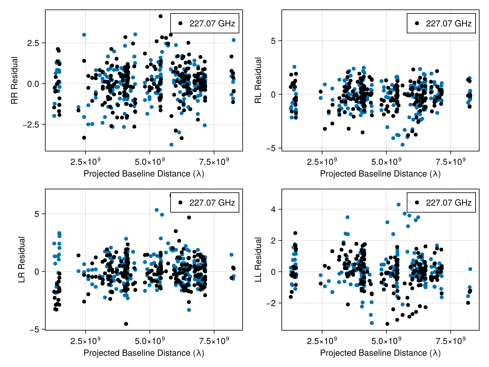

These look reasonable, although there may be some minor overfitting. Let's plot the results

julia

gpl = refinespatial(grid, 2)
img = intensitymap(skymodel(post, xopt), gpl)
fig = imageviz(
    img, adjust_length = true, colormap = :cmr_gothic, pcolormap = :rainbow1,
    pcolorrange = (0.0, 0.2), plot_total = false
);
fig |> DisplayAs.PNG |> DisplayAs.Text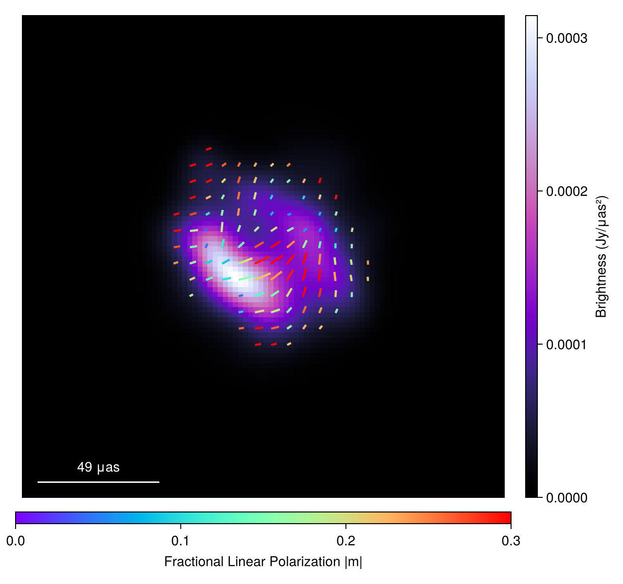

Note

The image looks a little noisy. This is an artifact of the MAP image. To get a publication quality image we recommend sampling from the posterior and averaging the samples. The results will be essentially identical to the results from EHTC VII.

We can also analyze the instrument model. For example, we can look at the gain ratios and products. To grab the ratios and products we can use the caltable function which will return analyze the gprat array and convert it to a uniform table. We can then plot the gain phases and amplitudes.

julia

gphase_ratio = caltable(xopt.instrument.gprat)
gamp_ratio = caltable(exp.(xopt.instrument.lgrat))

─────────┬───────────────────┬─────────────────────────────────────────────────────────────
      Ti │                Fr │    AA       AP       AZ       JC       LM       PV       SM
─────────┼───────────────────┼─────────────────────────────────────────────────────────────
 0.58 hr │ 227.070703125 GHz │ 1.006  missing  missing  missing  missing    1.048  missing
 0.73 hr │ 227.070703125 GHz │ 1.017    1.042  missing  missing  missing    1.023  missing
 0.88 hr │ 227.070703125 GHz │  1.07    0.982  missing  missing  missing    0.957  missing
  1.3 hr │ 227.070703125 GHz │ 0.987    1.036  missing  missing  missing    1.062  missing
 1.45 hr │ 227.070703125 GHz │ 1.004     1.01  missing  missing  missing     1.04  missing
 1.89 hr │ 227.070703125 GHz │  1.04    0.951  missing  missing  missing    1.018  missing
 2.04 hr │ 227.070703125 GHz │ 1.039    1.062    1.032  missing  missing    1.001  missing
 2.46 hr │ 227.070703125 GHz │  1.03    1.039    1.024  missing    1.042    1.023  missing
 2.61 hr │ 227.070703125 GHz │ 1.016    0.984    1.057  missing    1.066  missing  missing
 3.06 hr │ 227.070703125 GHz │ 1.027    1.019    1.043  missing    1.056    1.039  missing
 3.21 hr │ 227.070703125 GHz │ 1.002    0.995    1.053  missing    1.057  missing  missing
 3.62 hr │ 227.070703125 GHz │ 1.003    1.071    1.041  missing    1.047    1.059  missing
 3.78 hr │ 227.070703125 GHz │  1.02    0.975    1.058  missing    1.062    1.018  missing
 4.23 hr │ 227.070703125 GHz │ 0.994    0.956    1.045    0.867    1.042    1.056  missing
 4.37 hr │ 227.070703125 GHz │ 1.003    0.998    1.048     0.89    1.044    1.057  missing
 4.79 hr │ 227.070703125 GHz │ 1.004    0.911    1.061    0.981    1.037    1.043    0.878
 4.95 hr │ 227.070703125 GHz │ 0.998      1.0    1.049    1.015    1.081    1.047    0.925
 5.63 hr │ 227.070703125 GHz │ 1.022    0.994    1.025    1.037    1.038  missing    1.017
 6.15 hr │ 227.070703125 GHz │ 1.007    0.941    1.008    1.039    1.059  missing    0.988
 6.72 hr │ 227.070703125 GHz │ 0.995    1.025    1.047    1.047    1.055  missing    1.037
 7.23 hr │ 227.070703125 GHz │ 0.984    1.027    1.066    1.063    1.065  missing    1.076
 7.44 hr │ 227.070703125 GHz │ 0.998  missing    1.059    1.081    1.032  missing    1.052
─────────┴───────────────────┴─────────────────────────────────────────────────────────────

Plotting the phases first, we see large trends in the righ circular polarization phase. This is expected due to a lack of image centroid and the absense of absolute phase information in VLBI. However, the gain phase difference between the left and right circular polarization is stable and close to zero. This is expected since gain ratios are typically stable over the course of an observation and the constant offset was removed in the EHT calibration process.

julia

gphaseR = caltable(xopt.instrument.gpR)
fig = plotcaltable(gphaseR, gphase_ratio, labels = ["R Phase", "L/R Phase"]);
fig |> DisplayAs.PNG |> DisplayAs.Text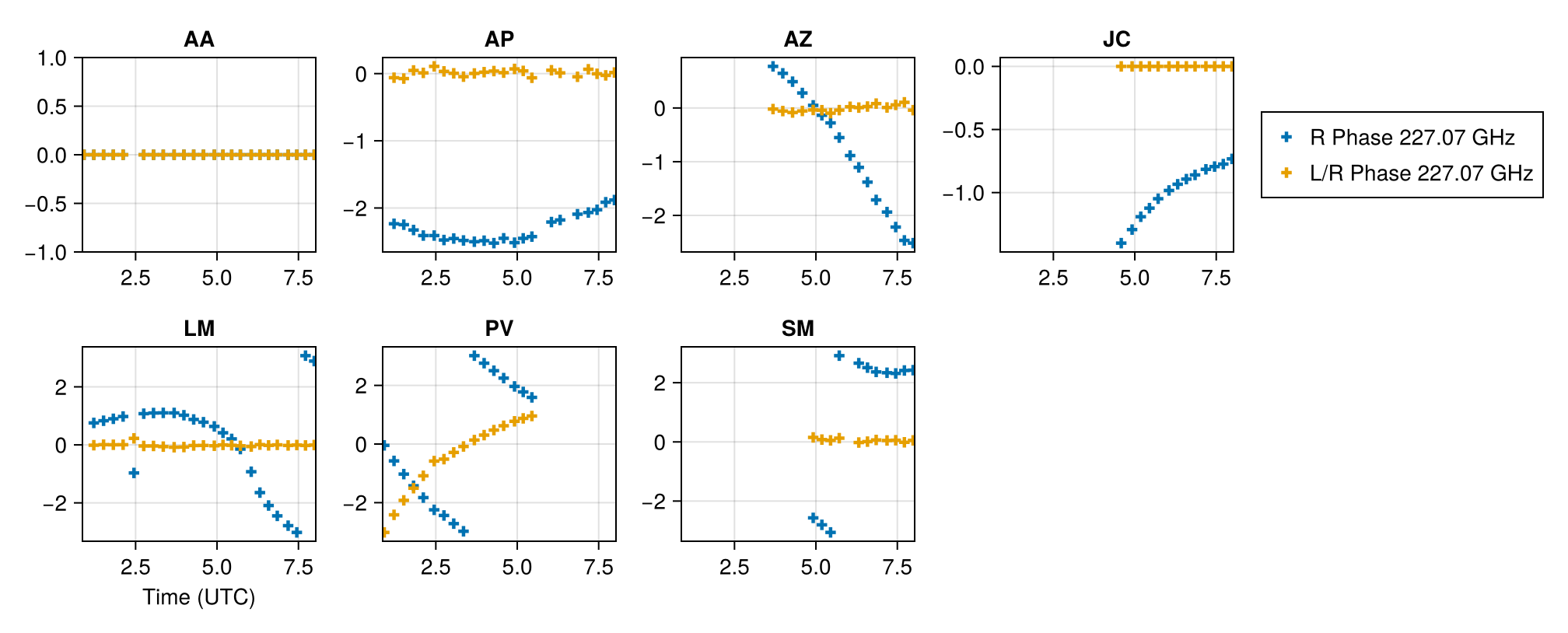

Moving to the amplitudes we see largely stable gain amplitudes on the right circular polarization except for LMT which is known and due to pointing issues during the 2017 observation. Again the gain ratios are stable and close to unity. Typically we expect that apriori calibration should make the gain ratios close to unity.

julia

gampr = caltable(exp.(xopt.instrument.lgR))
fig = plotcaltable(gampr, gamp_ratio, labels = ["R Amp", "L/R Amp"], axis_kwargs = (; limits = (nothing, (0.6, 1.3))));
fig |> DisplayAs.PNG |> DisplayAs.Text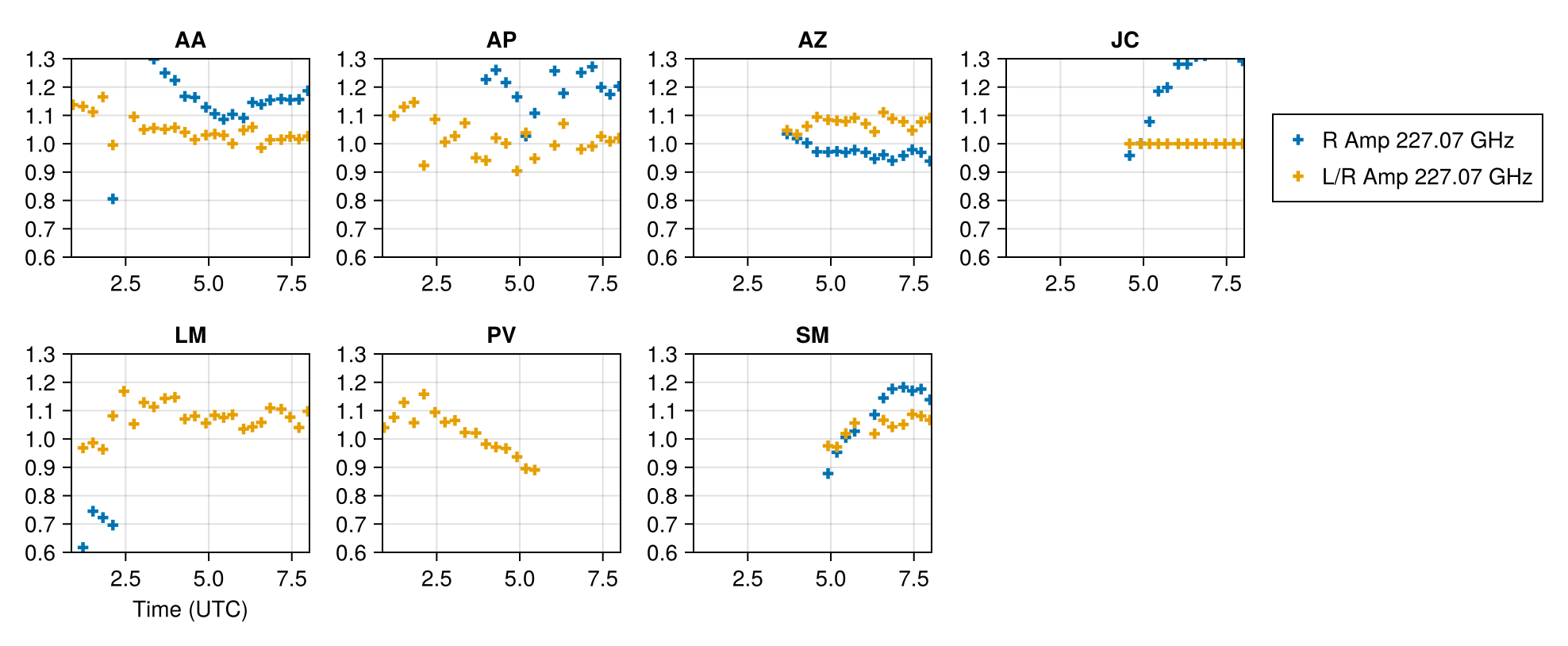

To sample from the posterior, you can then just use the sample function from AdvancedHMC like in the other imaging examples. For example

julia

using AdvancedHMC
chain = sample(rng, post, NUTS(0.8), 2_000, n_adapts = 1000, progress = true, initial_params = xopt)

This page was generated using Literate.jl.

Hamaker J.P, Bregman J.D., Sault R.J. (1996) [https://articles.adsabs.harvard.edu/pdf/1996A%26AS..117..137H] ↩︎
Pesce D. (2021) [https://ui.adsabs.harvard.edu/abs/2021AJ....161..178P/abstract] ↩︎

Polarized Image and Instrumental Modeling ​

Introduction to Polarized Imaging ​

Load the Data ​

Load the Data ​

Reconstructing the Image and Instrument Effects ​

Polarized Image and Instrumental Modeling

Introduction to Polarized Imaging

Load the Data

Load the Data

Reconstructing the Image and Instrument Effects