Loading Data into Comrade

The VLBI field does not have a standardized data format, and the EHT uses a particular uvfits format similar to the optical interferometry oifits format. In Comrade we read uvfits with the pure-Julia VLBIFiles.jl package, which avoids any Python dependency.

Once the data is loaded, we then convert the data into the tabular format Comrade expects.

To get started, we will load Comrade and CairoMakie to enable visualizations of the data.

using Comrade
using CairoMakie

We also load VLBIFiles to read the uvfits file. VLBIFiles re-exports VLBIData, so all of the data-table types (uvtable, Antenna, …) and the VLBI averaging namespace come along for free.

using VLBIFiles

We will use the 2017 public M87 data which can be downloaded from cyverse

uvd = VLBIFiles.load(
    VLBIFiles.UVData,
    joinpath(__DIR, "..", "..", "Data", "SR1_M87_2017_096_lo_hops_netcal_StokesI.uvfits")
)

VLBIFiles.UVData("/home/runner/work/Comrade.jl/Comrade.jl/examples/Data/SR1_M87_2017_096_lo_hops_netcal_StokesI.uvfits", VLBIFiles.UVHeader(SIMPLE  =                    T / conforms to FITS standard
BITPIX  =                  -32 / array data type
NAXIS   =                    7 / number of array dimensions
NAXIS1  =                    0
NAXIS2  =                    3
NAXIS3  =                    4
NAXIS4  =                    1
NAXIS5  =                    1
NAXIS6  =                    1
NAXIS7  =                    1
EXTEND  =                    T
GROUPS  =                    T / has groups
PCOUNT  =                    9 / number of parameters
GCOUNT  =                 8645 / number of groups
OBSRA   =    187.7059307575226
OBSDEC  =    12.39112323919932
OBJECT  = 'M87     '          
MJD     =              57849.0
DATE-OBS= '2017-04-06'        
BSCALE  =                  1.0
BZERO   =                  0.0
BUNIT   = 'JY      '          
VELREF  =                    3
EQUINOX = 'J2000   '          
ALTRPIX =                  1.0
ALTRVAL =                  0.0
TELESCOP= 'VLBA    '          
INSTRUME= 'VLBA    '          
OBSERVER= 'EHT     '          
CTYPE2  = 'COMPLEX '          
CRVAL2  =                  1.0
CDELT2  =                  1.0
CRPIX2  =                  1.0
CROTA2  =                  0.0
CTYPE3  = 'STOKES  '          
CRVAL3  =                 -1.0
CDELT3  =                 -1.0
CRPIX3  =                  1.0
CROTA3  =                  0.0
CTYPE4  = 'FREQ    '          
CRVAL4  =     2.27070703125e11
CDELT4  =              1.856e9
CRPIX4  =                  1.0
CROTA4  =                  0.0
CTYPE6  = 'RA      '          
CRVAL6  =    187.7059307575226
CDELT6  =                  1.0
CRPIX6  =                  1.0
CROTA6  =                  0.0
CTYPE7  = 'DEC     '          
CRVAL7  =    12.39112323919932
CDELT7  =                  1.0
CRPIX7  =                  1.0
CROTA7  =                  0.0
PTYPE1  = 'UU---SIN'          
PSCAL1  =  4.4039146672722e-12
PZERO1  =                  0.0
PTYPE2  = 'VV---SIN'          
PSCAL2  =  4.4039146672722e-12
PZERO2  =                  0.0
PTYPE3  = 'WW---SIN'          
PSCAL3  =  4.4039146672722e-12
PZERO3  =                  0.0
PTYPE4  = 'BASELINE'          
PSCAL4  =                  1.0
PZERO4  =                  0.0
PTYPE5  = 'DATE    '          
PSCAL5  =                  1.0
PZERO5  =                  0.0
PTYPE6  = 'DATE    '          
PSCAL6  =                  1.0
PZERO6  =                  0.0
PTYPE7  = 'INTTIM  '          
PSCAL7  =                  1.0
PZERO7  =                  0.0
PTYPE8  = 'TAU1    '          
PSCAL8  =                  1.0
PZERO8  =                  0.0
PTYPE9  = 'TAU2    '          
PSCAL9  =                  1.0
PZERO9  =                  0.0
HISTORY AIPS SORT ORDER='TB', "M87", Dates.Date("2017-04-06"), [:RR, :LL, :RL, :LR], 2.27070703125e11 Hz), VLBIFiles.FrequencyWindow[VLBIFiles.FrequencyWindow(1, 1, 2.270707f11 Hz, 1.856f9 Hz, 1, 1, 1.0f0)], VLBIFiles.AntArray[VLBIFiles.AntArray("VLBA", 2.270707f11 Hz, {1 = Antenna AA, 2 = Antenna AP, 3 = Antenna AZ, 4 = Antenna JC, 5 = Antenna LM, 6 = Antenna PV, 7 = Antenna SM, 8 = Antenna SR}, [0.0, 0.0, 0.0])])

We average the data over telescope scans by passing a time_average strategy on the data product. Note that the EHT data has been pre-calibrated so this averaging doesn't induce large coherence losses.

scan_avg = VLBI.GapBasedScans()
vis = extract_table(uvd, Visibilities(; time_average = scan_avg))                         # complex visibilities
amp = extract_table(uvd, VisibilityAmplitudes(; time_average = scan_avg))                 # visibility amplitudes
cphase = extract_table(uvd, ClosurePhases(; time_average = scan_avg))                        # minimal closure phases
lcamp = extract_table(uvd, LogClosureAmplitudes(; time_average = scan_avg))                 # minimal log-closure amplitudes

EHTObservationTable{Comrade.EHTLogClosureAmplitudeDatum{:I}}
  source:      M87
  mjd:         57849
  bandwidth:   1.856e9
  sites:       [:AA, :AP, :AZ, :JC, :LM, :PV, :SM]
  nsamples:    142

For polarization we load the file the same way; circular polarization is detected from the antenna feed types in the FITS table. We pass the antenna text file via arrayfile= so the telescope mount info is set correctly for the Coherencies extraction.

uvdp = VLBIFiles.load(
    VLBIFiles.UVData,
    joinpath(__DIR, "..", "..", "Data", "polarized_gaussian_all_corruptions.uvfits")
)
coh = extract_table(
    uvdp, Coherencies(;
        time_average = scan_avg,
        arrayfile = joinpath(__DIR, "..", "..", "Data", "array.txt"),
    )
)

EHTObservationTable{Comrade.EHTCoherencyDatum{Float64}}
  source:      17.761122472222223:-28.992189444444445
  mjd:         51544
  bandwidth:   1.0e9
  sites:       [:AA, :AP, :AZ, :JC, :LM, :PV, :SM]
  nsamples:    315

Warning

Always use our extract_cphase and extract_lcamp functions to find the closures eht-imaging will sometimes incorrectly calculate a non-redundant set of closures.

We can also recover the array used in the observation using

using DisplayAs
plotfields(coh, U, V, axis_kwargs = (xreversed = true,)) |> DisplayAs.PNG |> DisplayAs.Text # Plot the baseline coverage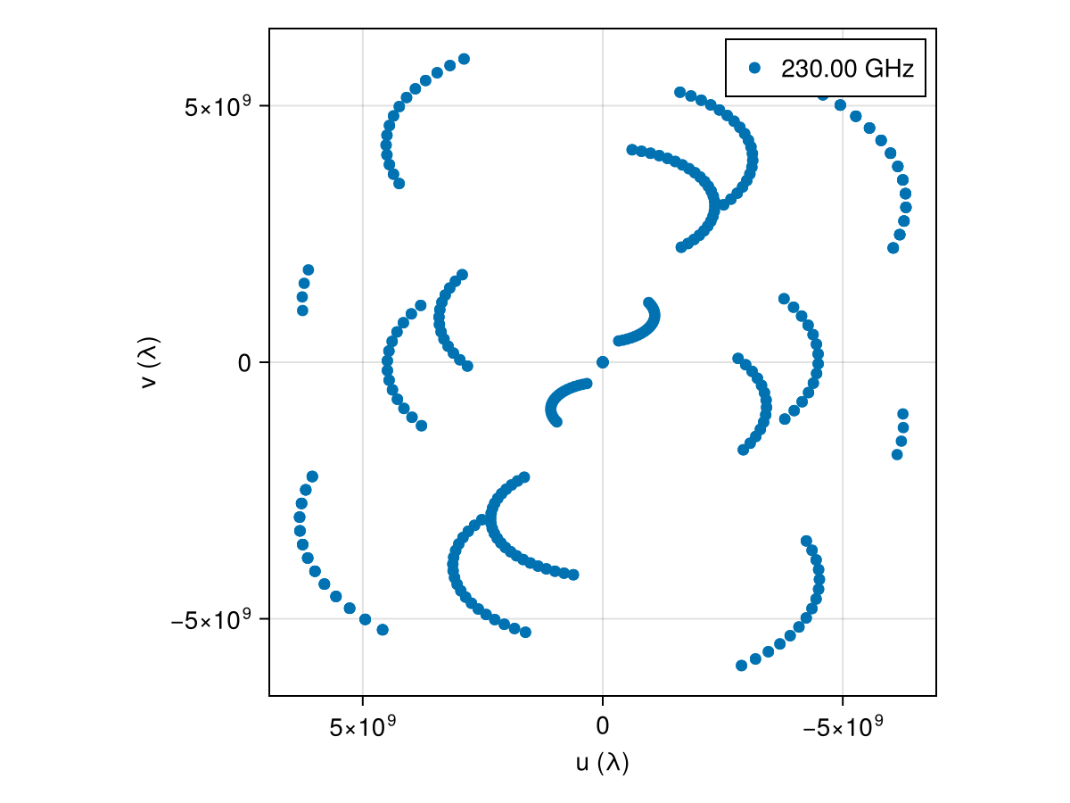

As of Comrade 0.11.7 Makie is the preferred plotting tool. For plotting data there are two classes of functions:

• baselineplot which gives complete control of plotting

• plotfields, axisfields which are more automated and limited but will automatically add labels, legends, titles etc.

fig = Figure(; size = (800, 600))
plotfields!(fig[1, 1], vis, uvdist, measurement)
plotfields!(fig[1, 2], amp, uvdist, measurement)
plotfields!(fig[2, 1], cphase, uvdist, measurement)
plotfields!(fig[2, 2], lcamp, uvdist, measurement)
fig |> DisplayAs.PNG |> DisplayAs.Text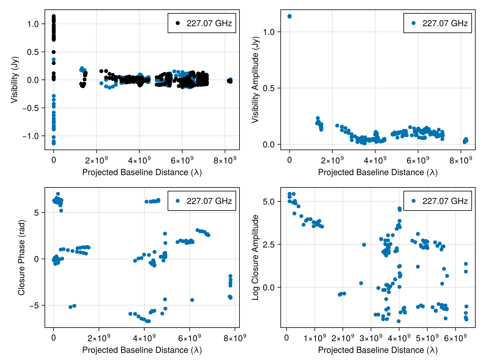

And also the coherency matrices. Since the data products are a matrix we need to plot each one separately.

fig = Figure(; size = (800, 600))
plotfields!(fig[1, 1], coh, uvdist, x -> measwnoise(x)[1, 1], axis_kwargs = (ylabel = "RR", xlabel = "uv distance (Gλ)"))
plotfields!(fig[2, 1], coh, uvdist, x -> measwnoise(x)[2, 1], axis_kwargs = (ylabel = "LR", xlabel = "uv distance (Gλ)"))
plotfields!(fig[1, 2], coh, uvdist, x -> measwnoise(x)[1, 2], axis_kwargs = (ylabel = "RL", xlabel = "uv distance (Gλ)"))
plotfields!(fig[2, 2], coh, uvdist, x -> measwnoise(x)[2, 2], axis_kwargs = (ylabel = "LL", xlabel = "uv distance (Gλ)"))
fig

You can also plot a single baseline

fig, ax = plotfields(coh, (:AA, :LM), Ti, x -> abs(measwnoise(x)[1, 1]), axis_kwargs = (; ylabel = "|RR|"))
ax2 = plotfields!(fig[1, 2], coh, (:LM, :AZ), Ti, x -> abs(measwnoise(x)[1, 1]), axis_kwargs = (; ylabel = "|RR|"))
fig

Finally, we provide a more low-level plotting function baselineplot which allows you to plot any field against any other field. This is what plotfields calls under the hood. However, it does not automatically add labels, legends, titles etc, but can add multiple baselines to the same plot.

fig, ax = baselineplot(coh, (:AA, :LM), Ti, x -> abs(measwnoise(x)[1, 1]), label = "AA-LM")
baselineplot!(ax, coh, (:LM, :AZ), Ti, x -> abs(measwnoise(x)[1, 1]), label = "LM-AZ")
ax.ylabel = "|RR|"
ax.xlabel = "Time (UTC)"
axislegend(ax)
fig

---

This page was generated using Literate.jl.