Imaging a Black Hole using only Closure Quantities

In this tutorial, we will create a preliminary reconstruction of the 2017 M87 data on April 6 using closure-only imaging. This tutorial is a general introduction to closure-only imaging in Comrade. For an introduction to simultaneous image and instrument modeling, see Stokes I Simultaneous Image and Instrument Modeling

Introduction to Closure Imaging

The EHT is one of the highest-resolution telescope ever created. Its resolution is equivalent to roughly tracking a hockey puck on the moon when viewing it from the earth. However, the EHT is also a unique interferometer. First, EHT data is incredibly sparse, the array is formed from only eight geographic locations around the planet. Second, the obseving frequency is much higher than traditional VLBI. Lastly, each site in the array is unique. They have different dishes, recievers, feeds, and electronics. Putting this all together implies that many of the common imaging techniques struggle to fit the EHT data and explore the uncertainty in both the image and instrument. One way to deal with some of these uncertainties is to not directly fit the data but instead fit closure quantities, which are independent of many of the instrumental effects that plague the data. The types of closure quantities are briefly described in Introduction to the VLBI Imaging Problem.

In this tutorial, we will do closure-only modeling of M87 to produce a posterior of images of M87.

To get started, we will load Comrade

using Comrade

Pyehtim loads eht-imaging using PythonCall this is necessary to load uvfits files currently.

using Pyehtim

For reproducibility we use a stable random number genreator

using StableRNGs
rng = StableRNG(123)

StableRNGs.LehmerRNG(state=0x000000000000000000000000000000f7)

Load the Data

To download the data visit https://doi.org/10.25739/g85n-f134 To load the eht-imaging obsdata object we do:

obs = ehtim.obsdata.load_uvfits(joinpath(__DIR, "..", "..", "Data", "SR1_M87_2017_096_lo_hops_netcal_StokesI.uvfits"))

Python: <ehtim.obsdata.Obsdata object at 0x7f55bdc41ae0>

Now we do some minor preprocessing:

• Scan average the data since the data have been preprocessed so that the gain phases are coherent.

• Add 2% systematic noise to deal with calibration issues such as leakage.

obs = scan_average(obs).add_fractional_noise(0.02)

Python: <ehtim.obsdata.Obsdata object at 0x7f55d4503dc0>

Now, we extract our closure quantities from the EHT data set. We flag now SNR points since the closure likelihood we use is only applicable to high SNR data.

dlcamp, dcphase  = extract_table(obs, LogClosureAmplitudes(;snrcut=3), ClosurePhases(;snrcut=3))

(EHTObservationTable{Comrade.EHTLogClosureAmplitudeDatum{:I}}
  source:      M87
  mjd:         57849
  bandwidth:   1.856e9
  sites:       [:AA, :AP, :AZ, :JC, :LM, :PV, :SM]
  nsamples:    128, EHTObservationTable{Comrade.EHTClosurePhaseDatum{:I}}
  source:      M87
  mjd:         57849
  bandwidth:   1.856e9
  sites:       [:AA, :AP, :AZ, :JC, :LM, :PV, :SM]
  nsamples:    152)

Note

Fitting low SNR closure data is complicated and requires a more sophisticated likelihood. If low-SNR data is very important we recommend fitting visibilties with a instrumental model.

Build the Model/Posterior

For our model, we will be using an image model that consists of a raster of point sources, convolved with some pulse or kernel to make a ContinuousImage. To define this model we define the standard two argument function sky that defines the sky model we want to fit. The first argument are the model parameters, and are typically a NamedTuple. The second argument defines the metadata for the model that is typically constant. For our model the constant metdata will just by the mean or prior image.

function sky(θ, metadata)
    (;fg, c, σimg) = θ
    (;mimg) = metadata
    # Apply the GMRF fluctuations to the image
    rast = apply_fluctuations(CenteredLR(), mimg, σimg.*c.params)
    m = ContinuousImage(((1-fg)).*rast, BSplinePulse{3}())
    # Force the image centroid to be at the origin
    x0, y0 = centroid(m)
    # Add a large-scale gaussian to deal with the over-resolved mas flux
    g = modify(Gaussian(), Stretch(μas2rad(250.0), μas2rad(250.0)), Renormalize(fg))
    return shifted(m, -x0, -y0) + g
end

sky (generic function with 1 method)

Now, let's set up our image model. The EHT's nominal resolution is 20-25 μas. Additionally, the EHT is not very sensitive to a larger field of views; typically, 60-80 μas is enough to describe the compact flux of M87. Given this, we only need to use a small number of pixels to describe our image.

npix = 32
fovxy = μas2rad(150.0)

7.27220521664304e-10

To define the image model we need to specify both the grid we will be using and the FT algorithm we will use, in this case the NFFT which is the most efficient.

grid = imagepixels(fovxy, fovxy, npix, npix)

RectiGrid(
executor: Serial()
Dimensions: 
↓ X Sampled{Float64} LinRange{Float64}(-3.5224744018114725e-10, 3.5224744018114725e-10, 32) ForwardOrdered Regular Points,
→ Y Sampled{Float64} LinRange{Float64}(-3.5224744018114725e-10, 3.5224744018114725e-10, 32) ForwardOrdered Regular Points
)

Now we need to specify our image prior. For this work we will use a Gaussian Markov Random field prior

using VLBIImagePriors, Distributions, DistributionsAD

Since we are using a Gaussian Markov random field prior we need to first specify our mean image. For this work we will use a symmetric Gaussian with a FWHM of 50 μas

fwhmfac = 2*sqrt(2*log(2))
mpr = modify(Gaussian(), Stretch(μas2rad(50.0)./fwhmfac))
imgpr = intensitymap(mpr, grid)
skymeta = (;mimg = imgpr./flux(imgpr));

In addition we want a reasonable guess for what the resolution of our image should be. For radio astronomy this is given by roughly the longest baseline in the image. To put this into pixel space we then divide by the pixel size.

beam = beamsize(dlcamp)
rat = (beam/(step(grid.X)))

5.326336637737519

To make the Gaussian Markov random field efficient we first precompute a bunch of quantities that allow us to scale things linearly with the number of image pixels. This drastically improves the usual N^3 scaling you get from usual Gaussian Processes.

crcache = ConditionalMarkov(GMRF, grid; order=1)

ConditionalMarkov(
Random Field: GaussMarkovRandomField
Graph: MarkovRandomFieldGraph{1}(
dims: (32, 32)
)
)

Now we can finally form our image prior. For this we use a heirarchical prior where the correlation length is given by a inverse gamma prior to prevent overfitting. Gaussian Markov random fields are extremly flexible models. To prevent overfitting it is common to use priors that penalize complexity. Therefore, we want to use priors that enforce similarity to our mean image, and prefer smoothness.

cprior = HierarchicalPrior(crcache, truncated(InverseGamma(1.0, -log(0.1)*rat); upper=2*npix))
prior = (c = cprior, σimg = Exponential(0.5), fg=Uniform(0.0, 1.0))

(c = HierarchicalPrior(
	map: 
	ConditionalMarkov(
Random Field: GaussMarkovRandomField
Graph: MarkovRandomFieldGraph{1}(
dims: (32, 32)
)
)	hyper prior: 
	Truncated(Distributions.InverseGamma{Float64}(
invd: Distributions.Gamma{Float64}(α=1.0, θ=0.0815371823902832)
θ: 12.264343342322437
)
; upper=64.0)

)
, σimg = Distributions.Exponential{Float64}(θ=0.5), fg = Distributions.Uniform{Float64}(a=0.0, b=1.0))

Putting this all together we can define our sky model.

skym = SkyModel(sky, prior, grid; metadata=skymeta)

 SkyModel
  with map: sky
   on grid: RectiGrid

Since we are fitting closures we do not need to include an instrument model, since the closure likelihood is approximately independent of gains in the high SNR limit.

post = VLBIPosterior(skym, dlcamp, dcphase)

VLBIPosterior
ObservedSkyModel
  with map: sky
   on grid: FourierDualDomainIdealInstrumentModelData Products: Comrade.EHTLogClosureAmplitudeDatumComrade.EHTClosurePhaseDatum

Reconstructing the Image

To reconstruct the image we will first use the MAP estimate. This is approach is basically a re-implentation of regularized maximum likelihood (RML) imaging. However, unlike traditional RML imaging we also fit the regularizer hyperparameters, thanks to our interpretation of as our imaging prior as a hierarchical model.

To optimize our posterior Comrade provides the comrade_opt function. To use this functionality a user first needs to import Optimization.jl and the optimizer of choice. In this tutorial we will use Optim.jl's L-BFGS optimizer, which is defined in the sub-package OptimizationOptimJL. We also need to import Zygote to allow for automatic differentiation.

using Optimization
using OptimizationOptimJL
using Zygote
xopt, sol = comrade_opt(post, LBFGS(), Optimization.AutoZygote(); maxiters=1000)

((sky = (c = (params = [-3.552061363378839e-7 -2.1637332401451175e-7 … -6.596223488366312e-6 -3.291043664832433e-6; 4.536212439952391e-6 6.304503312995015e-6 … -5.553767481733761e-6 -6.262021820937134e-6; … ; 1.773649842469953e-6 -3.569983284398999e-6 … -2.3266303873235853e-7 -3.677286563349164e-7; -1.8441541971158805e-7 -1.9723825075558274e-6 … -4.110176394903903e-6 -2.8812113906864284e-6], hyperparams = 0.013355381739163133), σimg = 49.96023032421502, fg = 0.14441433470237713),), retcode: Failure
u: [-3.552061363378839e-7, 4.536212439952391e-6, 9.140458629779937e-6, 1.0272529936678589e-5, 1.6502559123532872e-5, 2.023037510903949e-5, 8.463735280993437e-6, -1.6756323214687826e-5, -4.6130230631928994e-5, -6.668301950342051e-5  …  -2.7963414594596362e-5, -9.566510347458251e-6, 8.498059910986553e-8, 4.107940241514949e-6, 5.53815778544224e-6, -3.677286563349164e-7, -2.8812113906864284e-6, -8.47451023258422, 3.9112272954191885, -1.779099730767511]
Final objective value:     -2628.512741903953
)

First we will evaluate our fit by plotting the residuals

using Plots
p = residual(post, xopt)

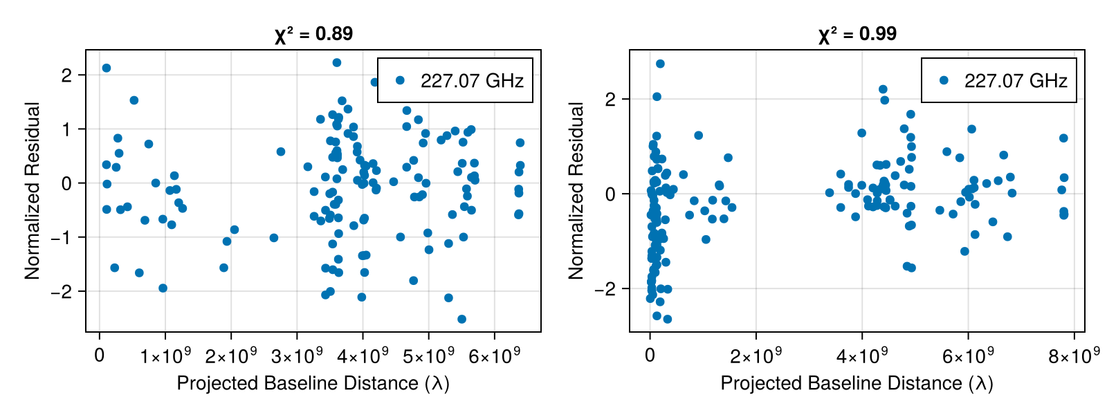
Now let's plot the MAP estimate.

import CairoMakie as CM
g = imagepixels(μas2rad(150.0), μas2rad(150.0), 100, 100)
img = intensitymap(skymodel(post, xopt), g)
fig = imageviz(img, size=(600, 500));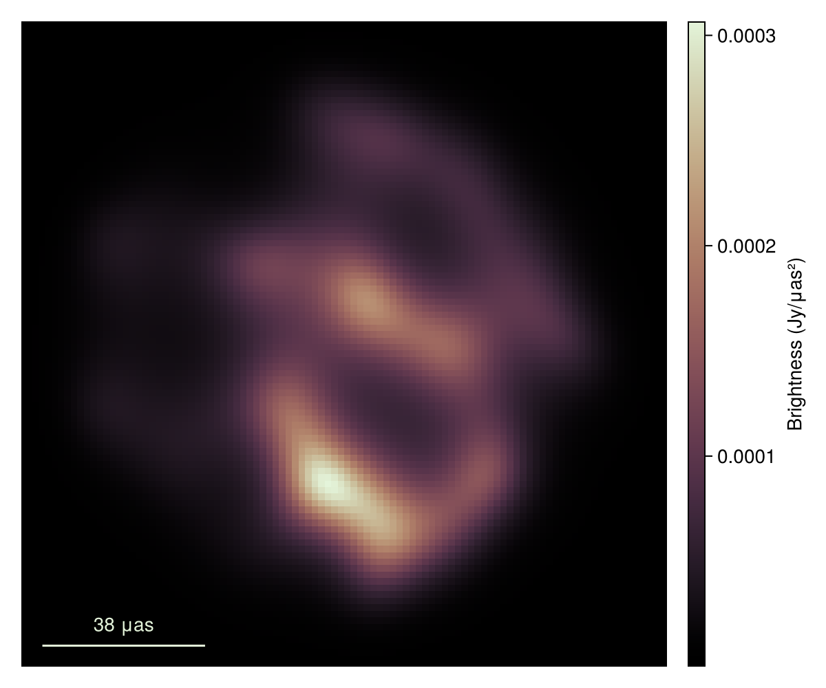

That doesn't look great. This is pretty common for the sparse EHT data. In this case the MAP often drastically overfits the data, producing a image filled with artifacts. In addition, we note that the MAP itself is not invariant to the model parameterization. Namely, if we changed our prior to use a fully centered parameterization we would get a very different image. Fortunately, these issues go away when we sample from the posterior, and construct expectations of the posterior, like the mean image.

To sample from the posterior we will use HMC and more specifically the NUTS algorithm. For information about NUTS see Michael Betancourt's notes.

Note

For our metric we use a diagonal matrix due to easier tuning.

using AdvancedHMC
chain = sample(post, NUTS(0.8), 700; n_adapts=500, progress=false, initial_params=xopt);

[ Info: Found initial step size 0.0001953125

Warning

This should be run for longer!

Now that we have our posterior, we can assess which parts of the image are strongly inferred by the data. This is rather unique to Comrade where more traditional imaging algorithms like CLEAN and RML are inherently unable to assess uncertainty in their reconstructions.

To explore our posterior let's first create images from a bunch of draws from the posterior

msamples = skymodel.(Ref(post), chain[501:2:end]);

The mean image is then given by

using StatsBase
imgs = intensitymap.(msamples, Ref(g))
mimg = mean(imgs)
simg = std(imgs)
fig = CM.Figure(;resolution=(700, 700));
axs = [CM.Axis(fig[i, j], xreversed=true, aspect=1) for i in 1:2, j in 1:2]
CM.image!(axs[1,1], mimg, colormap=:afmhot); axs[1, 1].title="Mean"
CM.image!(axs[1,2], simg./(max.(mimg, 1e-8)), colorrange=(0.0, 2.0), colormap=:afmhot);axs[1,2].title = "Std"
CM.image!(axs[2,1], imgs[1],   colormap=:afmhot);
CM.image!(axs[2,2], imgs[end], colormap=:afmhot);
CM.hidedecorations!.(axs)
fig |> DisplayAs.PNG |> DisplayAs.Text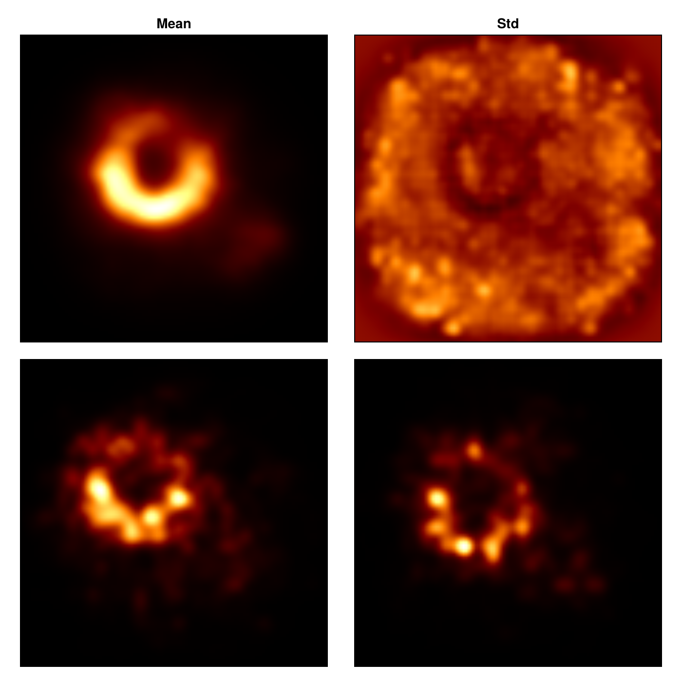

Now let's see whether our residuals look better.

p = Plots.plot(layout=(2,1));
for s in sample(chain[501:end], 10)
    residual!(post, s)
end
p |> DisplayAs.PNG |> DisplayAs.Text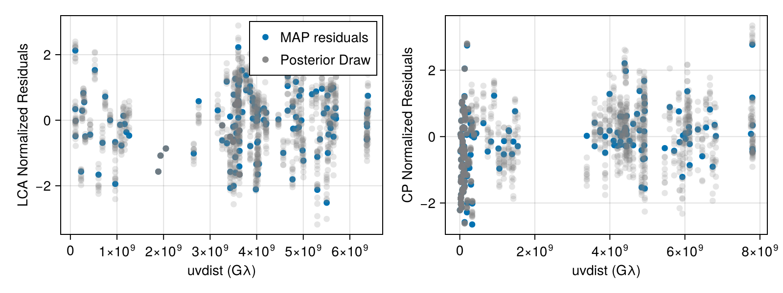

And viola, you have a quick and preliminary image of M87 fitting only closure products. For a publication-level version we would recommend

1. Running the chain longer and multiple times to properly assess things like ESS and R̂ (see Geometric Modeling of EHT Data)

2. Fitting gains. Typically gain amplitudes are good to 10-20% for the EHT not the infinite uncertainty closures implicitly assume

---

This page was generated using Literate.jl.