Geometric Modeling of EHT Data

Comrade has been designed to work with the EHT and ngEHT. In this tutorial, we will show how to reproduce some of the results from EHTC VI 2019.

In EHTC VI, they considered fitting simple geometric models to the data to estimate the black hole's image size, shape, brightness profile, etc. In this tutorial, we will construct a similar model and fit it to the data in under 50 lines of code (sans comments). To start, we load Comrade and some other packages we need.

using Comrade


using Pyehtim

For reproducibility we use a stable random number genreator

using StableRNGs
rng = StableRNG(42)

StableRNGs.LehmerRNG(state=0x00000000000000000000000000000055)

The next step is to load the data. We will use the publically available M 87 data which can be downloaded from cyverse. For an introduction to data loading, see Loading Data into Comrade.

obs = ehtim.obsdata.load_uvfits(joinpath(__DIR, "..", "..", "Data", "SR1_M87_2017_096_lo_hops_netcal_StokesI.uvfits"))

Python: <ehtim.obsdata.Obsdata object at 0x7f5812a280a0>

Now we will kill 0-baselines since we don't care about large-scale flux and since we know that the gains in this dataset are coherent across a scan, we make scan-average data

obs = Pyehtim.scan_average(obs.flag_uvdist(uv_min=0.1e9)).add_fractional_noise(0.02)

Python: <ehtim.obsdata.Obsdata object at 0x7f5802779270>

Now we extract the data products we want to fit

dlcamp, dcphase = extract_table(obs, LogClosureAmplitudes(;snrcut=3.0), ClosurePhases(;snrcut=3.0))

(EHTObservationTable{Comrade.EHTLogClosureAmplitudeDatum{:I}}
  source:      M87
  mjd:         57849
  bandwidth:   1.856e9
  sites:       [:AA, :AP, :AZ, :JC, :LM, :PV, :SM]
  nsamples:    94, EHTObservationTable{Comrade.EHTClosurePhaseDatum{:I}}
  source:      M87
  mjd:         57849
  bandwidth:   1.856e9
  sites:       [:AA, :AP, :AZ, :JC, :LM, :PV, :SM]
  nsamples:    118)

!!!warn We remove the low-snr closures since they are very non-gaussian. This can create rather large biases in the model fitting since the likelihood has much heavier tails that the usual Gaussian approximation.

For the image model, we will use a modified MRing, a infinitely thin delta ring with an azimuthal structure given by a Fourier expansion. To give the MRing some width, we will convolve the ring with a Gaussian and add an additional gaussian to the image to model any non-ring flux. Comrade expects that any model function must accept a named tuple and returns must always return an object that implements the VLBISkyModels Interface

function sky(θ, p)
    (;radius, width, ma, mp, τ, ξτ, f, σG, τG, ξG, xG, yG) = θ
    α = ma.*cos.(mp .- ξτ)
    β = ma.*sin.(mp .- ξτ)
    ring = f*smoothed(modify(MRing(α, β), Stretch(radius, radius*(1+τ)), Rotate(ξτ)), width)
    g = (1-f)*shifted(rotated(stretched(Gaussian(), σG, σG*(1+τG)), ξG), xG, yG)
    return ring + g
end

sky (generic function with 1 method)

To construct our likelihood p(V|M) where V is our data and M is our model, we use the RadioLikelihood function. The first argument of RadioLikelihood is always a function that constructs our Comrade model from the set of parameters θ.

We now need to specify the priors for our model. The easiest way to do this is to specify a NamedTuple of distributions:

using Distributions, VLBIImagePriors
prior = (
          radius = Uniform(μas2rad(10.0), μas2rad(30.0)),
          width = Uniform(μas2rad(1.0), μas2rad(10.0)),
          ma = (Uniform(0.0, 0.5), Uniform(0.0, 0.5)),
          mp = (Uniform(0, 2π), Uniform(0, 2π)),
          τ = Uniform(0.0, 1.0),
          ξτ= Uniform(0.0, π),
          f = Uniform(0.0, 1.0),
          σG = Uniform(μas2rad(1.0), μas2rad(100.0)),
          τG = Uniform(0.0, 1.0),
          ξG = Uniform(0.0, 1π),
          xG = Uniform(-μas2rad(80.0), μas2rad(80.0)),
          yG = Uniform(-μas2rad(80.0), μas2rad(80.0))
        )

(radius = Distributions.Uniform{Float64}(a=4.84813681109536e-11, b=1.454441043328608e-10), width = Distributions.Uniform{Float64}(a=4.84813681109536e-12, b=4.84813681109536e-11), ma = (Distributions.Uniform{Float64}(a=0.0, b=0.5), Distributions.Uniform{Float64}(a=0.0, b=0.5)), mp = (Distributions.Uniform{Float64}(a=0.0, b=6.283185307179586), Distributions.Uniform{Float64}(a=0.0, b=6.283185307179586)), τ = Distributions.Uniform{Float64}(a=0.0, b=1.0), ξτ = Distributions.Uniform{Float64}(a=0.0, b=3.141592653589793), f = Distributions.Uniform{Float64}(a=0.0, b=1.0), σG = Distributions.Uniform{Float64}(a=4.84813681109536e-12, b=4.84813681109536e-10), τG = Distributions.Uniform{Float64}(a=0.0, b=1.0), ξG = Distributions.Uniform{Float64}(a=0.0, b=3.141592653589793), xG = Distributions.Uniform{Float64}(a=-3.878509448876288e-10, b=3.878509448876288e-10), yG = Distributions.Uniform{Float64}(a=-3.878509448876288e-10, b=3.878509448876288e-10))

Note that for α and β we use a product distribution to signify that we want to use a multivariate uniform for the mring components α and β. In general the structure of the variables is specified by the prior. Note that this structure must be compatible with the model definition model(θ).

We can now construct our Sky model, which typically takes a model, prior and the on sky grid. Note that since our model is analytic the grid is not directly used when computing visibilities.

skym = SkyModel(sky, prior, imagepixels(μas2rad(200.0), μas2rad(200.0), 128, 128))

 SkyModel
  with map: sky
   on grid: RectiGrid

In this tutorial we will be using closure products as our data. As such we do not need to specify a instrument model, since for stokes I imaging, the likelihood is approximately invariant to the instrument model.

post = VLBIPosterior(skym, dlcamp, dcphase)

VLBIPosterior
ObservedSkyModel
  with map: sky
   on grid: FourierDualDomainIdealInstrumentModelData Products: Comrade.EHTLogClosureAmplitudeDatumComrade.EHTClosurePhaseDatum

Note

When fitting visibilities a instrument is required, and a reader can refer to Stokes I Simultaneous Image and Instrument Modeling.

This constructs a posterior density that can be evaluated by calling logdensityof. For example,

logdensityof(post, (sky = (radius = μas2rad(20.0),
                  width = μas2rad(10.0),
                  ma = (0.3, 0.3),
                  mp = (π/2, π),
                  τ = 0.1,
                  ξτ= π/2,
                  f = 0.6,
                  σG = μas2rad(50.0),
                  τG = 0.1,
                  ξG = 0.5,
                  xG = 0.0,
                  yG = 0.0),))

-4941.906769257601

Reconstruction

Now that we have fully specified our model, we now will try to find the optimal reconstruction of our model given our observed data.

Currently, post is in parameter space. Often optimization and sampling algorithms want it in some modified space. For example, nested sampling algorithms want the parameters in the unit hypercube. To transform the posterior to the unit hypercube, we can use the ascube function

cpost = ascube(post)

TransformedVLBIPosterior(
VLBIPosterior
ObservedSkyModel
  with map: sky
   on grid: FourierDualDomainIdealInstrumentModelData Products: Comrade.EHTLogClosureAmplitudeDatumComrade.EHTClosurePhaseDatum
Transform: Params to ℝ^14
)

If we want to flatten the parameter space and move from constrained parameters to (-∞, ∞) support we can use the asflat function

fpost = asflat(post)

TransformedVLBIPosterior(
VLBIPosterior
ObservedSkyModel
  with map: sky
   on grid: FourierDualDomainIdealInstrumentModelData Products: Comrade.EHTLogClosureAmplitudeDatumComrade.EHTClosurePhaseDatum
Transform: Params to ℝ^14
)

These transformed posterior expect a vector of parameters. For example, we can draw from the prior in our usual parameter space

p = prior_sample(rng, post)

(sky = (radius = 1.0476967761439489e-10, width = 1.3192620518421353e-11, ma = (0.48556673410322615, 0.3717248949271621), mp = (1.0742270769346676, 4.428237928961548), τ = 0.4410435910050243, ξτ = 2.5257522637778456, f = 0.772383948783141, σG = 3.450573255503277e-10, τG = 0.7393275279160691, ξG = 1.9708519781022533, xG = 1.067239797100682e-10, yG = -3.0224535970110963e-10),)

and then transform it to transformed space using T

logdensityof(cpost, Comrade.TV.inverse(cpost, p))
logdensityof(fpost, Comrade.TV.inverse(fpost, p))

-9995.571441536516

note that the log densit is not the same since the transformation has causes a jacobian to ensure volume is preserved.

Finding the Optimal Image

Typically, most VLBI modeling codes only care about finding the optimal or best guess image of our posterior post To do this, we will use Optimization.jl and specifically the BlackBoxOptim.jl package. For Comrade, this workflow is we use the comrade_opt function.

using Optimization
using OptimizationBBO
xopt, sol = comrade_opt(post, BBO_adaptive_de_rand_1_bin_radiuslimited(); maxiters=50_000);

Given this we can now plot the optimal image or the maximum a posteriori (MAP) image.

using DisplayAs
import CairoMakie as CM
g = imagepixels(μas2rad(200.0), μas2rad(200.0), 256, 256)
fig = imageviz(intensitymap(skymodel(post, xopt), g), colormap=:afmhot, size=(500, 400));
DisplayAs.Text(DisplayAs.PNG(fig))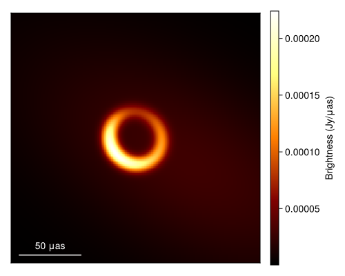

Quantifying the Uncertainty of the Reconstruction

While finding the optimal image is often helpful, in science, the most important thing is to quantify the certainty of our inferences. This is the goal of Comrade. In the language of Bayesian statistics, we want to find a representation of the posterior of possible image reconstructions given our choice of model and the data.

Comrade provides several sampling and other posterior approximation tools. To see the list, please see the Libraries section of the docs. For this example, we will be using Pigeons.jl which is a state-of-the-art parallel tempering sampler that enables global exploration of the posterior. For smaller dimension problems (< 100) we recommend using this sampler, especially if you have access to > 1 core.

using Pigeons
pt = pigeons(target=cpost, explorer=SliceSampler(), record=[traces, round_trip, log_sum_ratio], n_chains=16, n_rounds=8)

PT(checkpoint = false, ...)

That's it! To finish it up we can then plot some simple visual fit diagnostics. First we extract the MCMC chain for our posterior.

chain = sample_array(cpost, pt)

PosteriorSamples
  Samples size: (256,)
  sampler used: Pigeons
Mean
┌───────────────────────────────────────────────────────────────────────────────
│ sky                                                                          ⋯
│ @NamedTuple{radius::Float64, width::Float64, ma::Tuple{Float64, Float64}, mp ⋯
├───────────────────────────────────────────────────────────────────────────────
│ (radius = 9.61231e-11, width = 1.83847e-11, ma = (0.239993, 0.0639042), mp = ⋯
└───────────────────────────────────────────────────────────────────────────────
                                                                1 column omitted
Std. Dev.
┌───────────────────────────────────────────────────────────────────────────────
│ sky                                                                          ⋯
│ @NamedTuple{radius::Float64, width::Float64, ma::Tuple{Float64, Float64}, mp ⋯
├───────────────────────────────────────────────────────────────────────────────
│ (radius = 3.44783e-12, width = 2.7011e-12, ma = (0.0375602, 0.0237295), mp = ⋯
└───────────────────────────────────────────────────────────────────────────────
                                                                1 column omitted

First to plot the image we call

imgs = intensitymap.(skymodel.(Ref(post), sample(chain, 100)), Ref(g))
fig = imageviz(imgs[end], colormap=:afmhot)
DisplayAs.Text(DisplayAs.PNG(fig))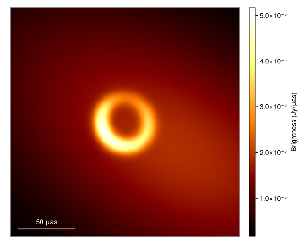

What about the mean image? Well let's grab 100 images from the chain, where we first remove the adaptation steps since they don't sample from the correct posterior distribution

meanimg = mean(imgs)
fig = imageviz(meanimg, colormap=:afmhot);
DisplayAs.Text(DisplayAs.PNG(fig))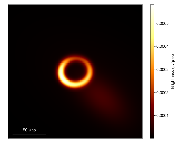

That looks similar to the EHTC VI, and it took us no time at all!. To see how well the model is fitting the data we can plot the model and data products

using Plots
p1 = Plots.plot(simulate_observation(post, xopt; add_thermal_noise=false)[1], label="MAP")
Plots.plot!(p1, dlcamp)
p2 = Plots.plot(simulate_observation(post, xopt; add_thermal_noise=false)[2], label="MAP")
Plots.plot!(p2, dcphase)
DisplayAs.Text(DisplayAs.PNG(Plots.plot(p1, p2, layout=(2,1))))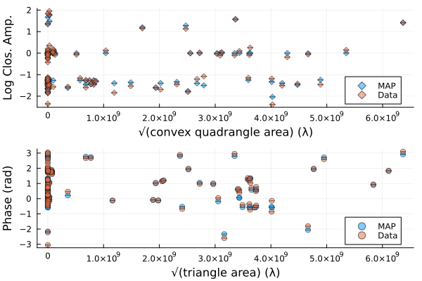

We can also plot random draws from the posterior predictive distribution. The posterior predictive distribution create a number of synthetic observations that are marginalized over the posterior.

p1 = Plots.plot(dlcamp);
p2 = Plots.plot(dcphase);
uva = uvdist.(datatable(dlcamp))
uvp = uvdist.(datatable(dcphase))
for i in 1:10
    mobs = simulate_observation(post, sample(chain, 1)[1])
    mlca = mobs[1]
    mcp  = mobs[2]
    Plots.scatter!(p1, uva, mlca[:measurement], color=:grey, label=:none, alpha=0.2)
    Plots.scatter!(p2, uvp, atan.(sin.(mcp[:measurement]), cos.(mcp[:measurement])), color=:grey, label=:none, alpha=0.2)
end
p = Plots.plot(p1, p2, layout=(2,1));
DisplayAs.Text(DisplayAs.PNG(p))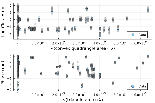

Finally, we can also put everything onto a common scale and plot the normalized residuals. The normalied residuals are the difference between the data and the model, divided by the data's error:

p = residual(post, chain[end]);
DisplayAs.Text(DisplayAs.PNG(p))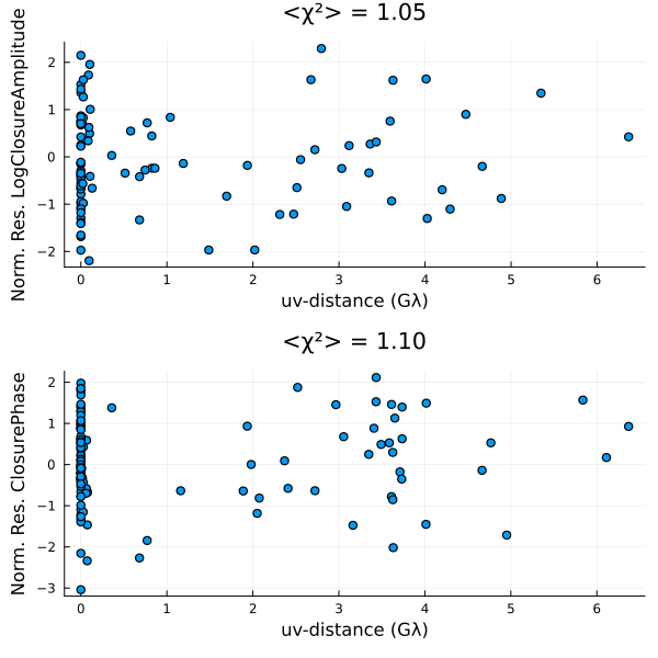

---

This page was generated using Literate.jl.