Polarized Image and Instrumental Modeling

In this tutorial, we will analyze a simulated simple polarized dataset to demonstrate Comrade's polarized imaging capabilities.

Introduction to Polarized Imaging

The EHT is a polarized interferometer. However, like all VLBI interferometers, it does not directly measure the Stokes parameters (I, Q, U, V). Instead, it measures components related to the electric field at the telescope along two directions using feeds. There are two types of feeds at telescopes: circular, which measure $R/L$ components of the electric field, and linear feeds, which measure $X/Y$ components of the electric field. Most sites in the EHT use circular feeds, meaning they measure the right (R) and left electric field (L) at each telescope. Although note that ALMA actually uses linear feeds. Currently Comrade has the ability to fit natively mixed polarization data however, the publically released EHT data has been converted to circular polarization. For a VLBI array whose feeds are purely circluar the coherency matrices are given by,

$$C_{ij}=\left(\begin{array}{cc}R{R}^{\ast }& R{L}^{\ast }\\ L{R}^{\ast }& L{L}^{\ast }\end{array}\right).$$

These coherency matrices are the fundamental object in interferometry and what the telescope observes. For a perfect interferometer, these circular coherency matrices are related to the usual Fourier transform of the stokes parameters by

$$\left(\begin{array}{c}\tilde{I}\\ \tilde{Q}\\ \tilde{U}\\ \tilde{V}\end{array}\right)=\frac{1}{2}\left(\begin{array}{c}R{R}^{\ast }+L{L}^{\ast }\\ R{L}^{\ast }+L{R}^{\ast }\\ i(L{R}^{\ast }-R{L}^{\ast })\\ R{R}^{\ast }-L{L}^{\ast }\end{array}\right).$$

Note

In this tutorial, we stick to circular feeds but Comrade has the capabilities to model linear (XX,XY, ...) and mixed basis coherencies (e.g., RX, RY, ...).

In reality, the measure coherencies are corrupted by both the atmosphere and the telescope itself. In Comrade we use the RIME formalism ^[1] to represent these corruptions, namely our measured coherency matrices $V_{ij}$ are given by

$$V_{ij}=J_i{C}_{ij}{J}_j^{†}$$

where $J$ is known as a Jones matrix and $ij$ denotes the baseline $ij$ with sites $i$ and $j$.

Comrade is highly flexible with how the Jones matrices are formed and provides several convenience functions that parameterize standard Jones matrices. These matrices include:

• JonesG which builds the set of complex gain Jones matrices

$$G=\left(\begin{array}{cc}{g}_a& 0\\ 0& g_b\end{array}\right)$$

• JonesD which builds the set of complex d-terms Jones matrices

$$D=\left(\begin{array}{cc}1& d_a\\ d_b& 1\end{array}\right)$$

• JonesR is the basis transform matrix $T$. This transformation is special and combines two things using the decomposition $T=FB$. The first, $B$, is the transformation from some reference basis to the observed coherency basis (this allows for mixed basis measurements). The second is the feed rotation, $F$, that transforms from some reference axis to the axis of the telescope as the source moves in the sky. The feed rotation matrix F for circular feeds in terms of the per station feed rotation angle $\phi$ is

$$F=\left(\begin{array}{cc}{e}^{-i\phi }& 0\\ 0& e^{i\phi }\end{array}\right)$$

In the rest of the tutorial, we are going to solve for all of these instrument model terms in while re-creating the polarized image from the first EHT results on M87.

Load the Data

To get started we will load Comrade

using Comrade

Load the Data

using Pyehtim

For reproducibility we use a stable random number genreator

using StableRNGs
rng = StableRNG(42)

StableRNGs.LehmerRNG(state=0x00000000000000000000000000000055)

Now we will load some synthetic polarized data.

fname = Base.download("https://de.cyverse.org/anon-files/iplant/home/shared/commons_repo/curated/EHTC_M87pol2017_Nov2023/hops_data/April11/SR2_M87_2017_101_lo_hops_ALMArot.uvfits",
                      joinpath(__DIR, "m87polarized.uvfits")
                    )
obs = Pyehtim.load_uvfits_and_array(
        fname,
        joinpath(__DIR, "..", "..", "Data", "array.txt"), polrep="circ")

Python: <ehtim.obsdata.Obsdata object at 0x7f58027f1870>

Notice that, unlike other non-polarized tutorials, we need to include a second argument. This is the array file of the observation and is required to determine the feed rotation of the array.

Now we scan average the data since the data to boost the SNR and reduce the total data volume.

obs = scan_average(obs).add_fractional_noise(0.01).flag_uvdist(uv_min=0.1e9)

Python: <ehtim.obsdata.Obsdata object at 0x7f57dfe3ee60>

Now we extract our observed/corrupted coherency matrices.

dvis = extract_table(obs, Coherencies())

EHTObservationTable{Comrade.EHTCoherencyDatum{Float64}}
  source:      M87
  mjd:         57854
  bandwidth:   1.856e9
  sites:       [:AA, :AP, :AZ, :JC, :LM, :PV, :SM]
  nsamples:    189

##Building the Model/Posterior

To build the model, we first break it down into two parts:

1. The image or sky model. In Comrade, all polarized image models are written in terms of the Stokes parameters. In this tutorial, we will use a polarized image model based on Pesce (2021)^[2], and parameterizes each pixel in terms of the Poincare sphere. This parameterization ensures that we have all the physical properties of stokes parameters. Note that we also have a parameterization in terms of hyperbolic trig functions VLBISkyModels.PolExp2Map

2. The instrument model. The instrument model specifies the model that describes the impact of instrumental and atmospheric effects. We will be using the $J=GDR$ decomposition we described above. However, to parameterize the R/L complex gains, we will be using a gain product and ratio decomposition. The reason for this decomposition is that in realistic measurements, the gain ratios and products have different temporal characteristics. Namely, many of the EHT observations tend to demonstrate constant R/L gain ratios across an nights observations, compared to the gain products, which vary every scan. Additionally, the gain ratios tend to be smaller (i.e., closer to unity) than the gain products. Using this apriori knowledge, we can build this into our model and reduce the total number of parameters we need to model.

First we specify our sky model. As always Comrade requires this to be a two argument function where the first argument is typically a NamedTuple of parameters we will fit and the second are additional metadata required to build the model.

using StatsFuns: logistic
function sky(θ, metadata)
    (;c, σ, p, p0, pσ, angparams) = θ
    (;mimg, ftot) = metadata
    # Build the stokes I model
    rast = apply_fluctuations(CenteredLR(), mimg, σ.*c.params)
    brast = baseimage(rast)
    brast .= ftot.*brast
    # The total polarization fraction is modeled in logit space so we transform it back
    pim = logistic.(p0 .+ pσ.*p.params)
    # Build our IntensityMap
    pmap = PoincareSphere2Map(rast, pim, angparams)
    # Construct the actual image model which uses a third order B-spline pulse
    m = ContinuousImage(pmap, BSplinePulse{3}())
    # Finally find the image centroid and shift it to be at the center
    x0, y0 = centroid(pmap)
    ms = shifted(m, -x0, -y0)
    return ms
end

sky (generic function with 1 method)

Now, we define the model metadata required to build the model. We specify our image grid and cache model needed to define the polarimetric image model. Our image will be a 10x10 raster with a 60μas FOV.

using Distributions
using VLBIImagePriors
fovx = μas2rad(200.0)
fovy = μas2rad(200.0)
nx = ny = 32
grid = imagepixels(fovx, fovy, nx, ny)

fwhmfac = 2*sqrt(2*log(2))
mpr  = modify(Gaussian(), Stretch(μas2rad(50.0)./fwhmfac))
mimg = intensitymap(mpr, grid)

╭───────────────────────────────╮
│ 32×32 IntensityMap{Float64,2} │
├───────────────────────────────┴──────────────────────────────────────── dims ┐
  ↓ X Sampled{Float64} LinRange{Float64}(-4.69663253574863e-10, 4.69663253574863e-10, 32) ForwardOrdered Regular Points,
  → Y Sampled{Float64} LinRange{Float64}(-4.69663253574863e-10, 4.69663253574863e-10, 32) ForwardOrdered Regular Points
├──────────────────────────────────────────────────────────────────── metadata ┤
  ComradeBase.NoHeader()
└──────────────────────────────────────────────────────────────────────────────┘
  ↓ →          -4.69663e-10  -4.39362e-10  …  4.39362e-10  4.69663e-10
 -4.69663e-10   1.25675e-11   4.60978e-11     4.60978e-11  1.25675e-11
 -4.39362e-10   4.60978e-11   1.69087e-10     1.69087e-10  4.60978e-11
 -4.09062e-10   1.55054e-10   5.6874e-10      5.6874e-10   1.55054e-10
  ⋮                                        ⋱               
  4.09062e-10   1.55054e-10   5.6874e-10   …  5.6874e-10   1.55054e-10
  4.39362e-10   4.60978e-11   1.69087e-10     1.69087e-10  4.60978e-11
  4.69663e-10   1.25675e-11   4.60978e-11     4.60978e-11  1.25675e-11

For the image metadata we specify the grid and the total flux of the image, which is 1.0. Note that we specify the total flux out front since it is degenerate with an overall shift in the gain amplitudes.

skymeta = (; mimg=mimg./flux(mimg), ftot=0.6)

(mimg = [1.2567547416996487e-11 4.60979671782088e-11 … 4.60979671782088e-11 1.2567547416996487e-11; 4.60979671782088e-11 1.690880891437348e-10 … 1.690880891437348e-10 4.60979671782088e-11; … ; 4.60979671782088e-11 1.690880891437348e-10 … 1.690880891437348e-10 4.60979671782088e-11; 1.2567547416996487e-11 4.60979671782088e-11 … 4.60979671782088e-11 1.2567547416996487e-11], ftot = 0.6)

We use again use a GMRF prior similar to the Imaging a Black Hole using only Closure Quantities tutorial for the log-ratio transformed image. We use the same correlated image prior for the inverse-logit transformed total polarization. The mean total polarization fraction p0 is centered at -2.0 with a standard deviation of 2.0 which logit transformed puts most of the prior mass < 0.8 fractional polarization. The standard deviation of the total polarization fraction pσ again uses a Half-normal process. The angular parameters of the polarizaton are given by a uniform prior on the sphere.

cprior = corr_image_prior(grid, dvis)
skyprior = (
    c = cprior,
    σ  = Exponential(0.1),
    p  = cprior,
    p0 = Normal(-2.0, 2.0),
    pσ =  truncated(Normal(0.0, 1.0); lower=0.01),
    angparams = ImageSphericalUniform(nx, ny),
    )

skym = SkyModel(sky, skyprior, grid; metadata=skymeta)

 SkyModel
  with map: sky
   on grid: RectiGrid

Now we build the instrument model. Due to the complexity of VLBI the instrument model is critical to the success of imaging and getting reliable results. For this example we will use the standard instrument model used in polarized EHT analyses expressed in the RIME formalism. Our Jones decomposition will be given by GDR, where G are the complex gains, D are the d-terms, and R is what we call the ideal instrument response, which is how an ideal interferometer using the feed basis we observe relative to some reference basis.

Given the possible flexibility in different parameterizations of the individual Jones matrices each Jones matrix requires the user to specify a function that converts from parameters to specific parameterization f the jones matrices.

For the complex gain matrix, we used the JonesG jones matrix. The first argument is now a function that converts from the parameters to the complex gain matrix. In this case, we will use a amplitude and phase decomposition of the complex gain matrix. Note that since the gain matrix is a diagonal 2x2 matrix the function must return a 2-element tuple. The first element of the tuple is the gain for the first polarization feed (R) and the second is the gain for the second polarization feed (L).

function fgain(x)
    gR = exp(x.lgR + 1im*x.gpR)
    gL = gR*exp(x.lgrat + 1im*x.gprat)
    return gR, gL
end
G = JonesG(fgain)

JonesG{typeof(Main.fgain)}(Main.fgain)

Similarly we provide a JonesD function for the leakage terms. Since we assume that we are in the small leakage limit, we will use the decomposition 1 d1 d2 1 Therefore, there are 2 free parameters for the JonesD our parameterization function must return a 2-element tuple. For d-terms we will use a re-im parameterization.

function fdterms(x)
    dR = complex(x.dRx, x.dRy)
    dL = complex(x.dLx, x.dLy)
    return dR, dL
end
D = JonesD(fdterms)

JonesD{typeof(Main.fdterms)}(Main.fdterms)

Finally we define our response Jones matrix. This matrix is a basis transform matrix plus the feed rotation angle for each station. These are typically set by the telescope so there are no free parameters, so no parameterization is necessary.

R = JonesR(;add_fr=true)

JonesR{Nothing}(nothing, true)

Finally, we build our total Jones matrix by using the JonesSandwich function. The first argument is a function that specifies how to combine each Jones matrix. In this case we will use the standard decomposition J = adjoint(R)_G_D*R, where we need to apply the adjoint of the feed rotaion matrix R because the data has feed rotation calibration.

js(g,d,r) = adjoint(r)*g*d*r
J = JonesSandwich(js, G, D, R)

JonesSandwich{Base.Splat{typeof(Main.js)}, Tuple{JonesG{typeof(Main.fgain)}, JonesD{typeof(Main.fdterms)}, JonesR{Nothing}}}(splat(js), (JonesG{typeof(Main.fgain)}(Main.fgain), JonesD{typeof(Main.fdterms)}(Main.fdterms), JonesR{Nothing}(nothing, true)))

Note

This is a general note that for arrays with non-zero leakage, feed rotation calibration does not remove the impact of feed rotations on the instrument model. That is, when modeling feed rotation must be taken into account. This is because the R and D matrices are not commutative. Therefore, to recover the correct instrumental terms we must include the feed rotation calibration in the instrument model. This is not ideal when doing polarized modeling, especially for interferometers using a mixture of linear and circular feeds. For linear feeds R does not commute with G or D and applying feed rotation calibration before solving for gains can mix gains and leakage with feed rotation calibration terms breaking many of the typical assumptions about the stabilty of different instrument effects.

For the instrument prior, we will use a simple IID prior for the complex gains and d-terms. The IIDSitePrior function specifies that each site has the same prior and each value is independent on some time segment. The current time segments are

• ScanSeg() which specifies each scan has an independent value

• TrackSeg() which says that the value is constant over the track.

• IntegSeg() which says that the value changes each integration time

For the released EHT data, the calibration procedure makes gains stable over each scan so we use ScanSeg for those quantities. The d-terms are typically stable over the track so we use TrackSeg for those.

intprior = (
    lgR  = ArrayPrior(IIDSitePrior(ScanSeg(), Normal(0.0, 0.2))),
    lgrat= ArrayPrior(IIDSitePrior(ScanSeg(), Normal(0.0, 0.01))),
    gpR  = ArrayPrior(IIDSitePrior(ScanSeg(), DiagonalVonMises(0.0, inv(π^2))); refant=SEFDReference(0.0), phase=true),
    gprat= ArrayPrior(IIDSitePrior(ScanSeg(), DiagonalVonMises(0.0, inv(0.1^2))); refant = SingleReference(:AA, 0.0), phase=false),
    dRx  = ArrayPrior(IIDSitePrior(TrackSeg(), Normal(0.0, 0.2))),
    dRy  = ArrayPrior(IIDSitePrior(TrackSeg(), Normal(0.0, 0.2))),
    dLx  = ArrayPrior(IIDSitePrior(TrackSeg(), Normal(0.0, 0.2))),
    dLy  = ArrayPrior(IIDSitePrior(TrackSeg(), Normal(0.0, 0.2))),
)

(lgR = ArrayPrior{IIDSitePrior{ScanSeg, Distributions.Normal{Float64}}, Base.Pairs{Symbol, Union{}, Tuple{}, @NamedTuple{}}, NoReference, Nothing}(IIDSitePrior{ScanSeg, Distributions.Normal{Float64}}(ScanSeg(), Distributions.Normal{Float64}(μ=0.0, σ=0.2)), Base.Pairs{Symbol, Union{}, Tuple{}, @NamedTuple{}}(), NoReference(), false, nothing), lgrat = ArrayPrior{IIDSitePrior{ScanSeg, Distributions.Normal{Float64}}, Base.Pairs{Symbol, Union{}, Tuple{}, @NamedTuple{}}, NoReference, Nothing}(IIDSitePrior{ScanSeg, Distributions.Normal{Float64}}(ScanSeg(), Distributions.Normal{Float64}(μ=0.0, σ=0.01)), Base.Pairs{Symbol, Union{}, Tuple{}, @NamedTuple{}}(), NoReference(), false, nothing), gpR = ArrayPrior{IIDSitePrior{ScanSeg, DiagonalVonMises{Float64, Float64, Float64}}, Base.Pairs{Symbol, Union{}, Tuple{}, @NamedTuple{}}, SEFDReference{Float64}, Nothing}(IIDSitePrior{ScanSeg, DiagonalVonMises{Float64, Float64, Float64}}(ScanSeg(), DiagonalVonMises{Float64, Float64, Float64}(μ=0.0, κ=0.10132118364233778, lnorm=-1.739120733481688)), Base.Pairs{Symbol, Union{}, Tuple{}, @NamedTuple{}}(), SEFDReference{Float64}(0.0, 0), true, nothing), gprat = ArrayPrior{IIDSitePrior{ScanSeg, DiagonalVonMises{Float64, Float64, Float64}}, Base.Pairs{Symbol, Union{}, Tuple{}, @NamedTuple{}}, SingleReference{Float64}, Nothing}(IIDSitePrior{ScanSeg, DiagonalVonMises{Float64, Float64, Float64}}(ScanSeg(), DiagonalVonMises{Float64, Float64, Float64}(μ=0.0, κ=99.99999999999999, lnorm=1.3823902436480708)), Base.Pairs{Symbol, Union{}, Tuple{}, @NamedTuple{}}(), SingleReference{Float64}(:AA, 0.0), false, nothing), dRx = ArrayPrior{IIDSitePrior{TrackSeg, Distributions.Normal{Float64}}, Base.Pairs{Symbol, Union{}, Tuple{}, @NamedTuple{}}, NoReference, Nothing}(IIDSitePrior{TrackSeg, Distributions.Normal{Float64}}(TrackSeg(), Distributions.Normal{Float64}(μ=0.0, σ=0.2)), Base.Pairs{Symbol, Union{}, Tuple{}, @NamedTuple{}}(), NoReference(), false, nothing), dRy = ArrayPrior{IIDSitePrior{TrackSeg, Distributions.Normal{Float64}}, Base.Pairs{Symbol, Union{}, Tuple{}, @NamedTuple{}}, NoReference, Nothing}(IIDSitePrior{TrackSeg, Distributions.Normal{Float64}}(TrackSeg(), Distributions.Normal{Float64}(μ=0.0, σ=0.2)), Base.Pairs{Symbol, Union{}, Tuple{}, @NamedTuple{}}(), NoReference(), false, nothing), dLx = ArrayPrior{IIDSitePrior{TrackSeg, Distributions.Normal{Float64}}, Base.Pairs{Symbol, Union{}, Tuple{}, @NamedTuple{}}, NoReference, Nothing}(IIDSitePrior{TrackSeg, Distributions.Normal{Float64}}(TrackSeg(), Distributions.Normal{Float64}(μ=0.0, σ=0.2)), Base.Pairs{Symbol, Union{}, Tuple{}, @NamedTuple{}}(), NoReference(), false, nothing), dLy = ArrayPrior{IIDSitePrior{TrackSeg, Distributions.Normal{Float64}}, Base.Pairs{Symbol, Union{}, Tuple{}, @NamedTuple{}}, NoReference, Nothing}(IIDSitePrior{TrackSeg, Distributions.Normal{Float64}}(TrackSeg(), Distributions.Normal{Float64}(μ=0.0, σ=0.2)), Base.Pairs{Symbol, Union{}, Tuple{}, @NamedTuple{}}(), NoReference(), false, nothing))

Finally, we can build our instrument model which takes a model for the Jones matrix J and priors for each term in the Jones matrix.

intmodel = InstrumentModel(J, intprior)

InstrumentModel
  with Jones:  JonesSandwich
  with reference basis: CirBasis()

intmodel = InstrumentModel(JonesR(;add_fr=true)) Putting it all together, we form our likelihood and posterior objects for optimization and sampling, and specifying to use Enzyme.Reverse with runtime activity for AD.

using Enzyme
post = VLBIPosterior(skym, intmodel, dvis; admode=set_runtime_activity(Enzyme.Reverse))

VLBIPosterior
ObservedSkyModel
  with map: sky
   on grid: FourierDualDomainObservedInstrumentModel
  with Jones:  JonesSandwich
  with reference basis: CirBasis()Data Products: Comrade.EHTCoherencyDatum

Reconstructing the Image and Instrument Effects

To sample from this posterior, it is convenient to move from our constrained parameter space to an unconstrained one (i.e., the support of the transformed posterior is (-∞, ∞)). This transformation is done using the asflat function.

tpost = asflat(post)

TransformedVLBIPosterior(
VLBIPosterior
ObservedSkyModel
  with map: sky
   on grid: FourierDualDomainObservedInstrumentModel
  with Jones:  JonesSandwich
  with reference basis: CirBasis()Data Products: Comrade.EHTCoherencyDatum
Transform: Params to ℝ^5689
)

We can also query the dimension of our posterior or the number of parameters we will sample.

Warning

This can often be different from what you would expect. This difference is especially true when using angular variables, where we often artificially increase the dimension of the parameter space to make sampling easier.

Now we optimize. Unlike other imaging examples, we move straight to gradient optimizers due to the higher dimension of the space. In addition the only AD package that can currently work with the polarized Comrade posterior is Enzyme.

using Optimization
using OptimizationOptimisers
xopt, sol = comrade_opt(post, Optimisers.Adam();
                        initial_params=prior_sample(rng, post), maxiters=25_000)

((sky = (c = (params = [1.312135887948237e-5 7.779690990799818e-7 … 3.933772155280565e-6 8.926187952710962e-6; -6.147811125006939e-6 3.105066347571787e-5 … 2.7707913345189492e-5 4.7915198151963145e-6; … ; -1.1780733212842579e-5 3.309903479261183e-5 … 2.2278701494308418e-5 7.852508438835115e-6; 1.9261185216954923e-5 -1.131223728040669e-5 … 4.669224279147073e-6 4.6751316833794515e-6], hyperparams = 1.0048588729531824), σ = 3.119557848590806, p = (params = [2.053384305069579e-5 -1.9773279216812752e-5 … 4.456542078945282e-5 -4.209300188690556e-5; -2.1301071700389724e-5 2.1716850859860914e-5 … -4.6309365322091066e-5 4.4593942707489157e-5; … ; -8.41794545358863e-6 9.00014404623846e-6 … 9.786728998069851e-7 -1.8725708633276458e-7; 9.124680671763283e-6 -9.057509218856604e-6 … -4.7113824765198044e-7 3.735479484564707e-7], hyperparams = 1.0041907035319029), p0 = 2.267030592649417, pσ = 1.0081718406325224, angparams = ([-0.03100377236122835 0.8767464909108951 … 0.18907543547012107 0.3158218187549682; 0.7198504266450012 -0.3221556509016461 … -0.3375723507774074 0.7910639669968237; … ; -0.4401655393885174 0.0430502928197741 … -0.34061480120494475 -0.46049312298180206; -0.7210392160814914 -0.6409228656519969 … 0.31268776823427835 -0.9899771209193475], [-0.997187366052602 -0.44325037134445755 … 0.11525035762567888 -0.8878571960919576; -0.11689591580408541 -0.9456787918555047 … 0.6393426588528967 0.4990205256787177; … ; -0.8905653975890357 -0.8478259580787848 … 0.8985716908323762 -0.8047027128409562; -0.6659022258445402 -0.33242297636784923 … 0.8850922926586622 -0.11386278777306508], [0.06823579034822484 0.18666734845288993 … -0.9751757968535402 -0.334613475738846; -0.684215396002848 0.04367332397298774 … -0.690858793503798 0.3538309131076374; … ; 0.11466285602538637 0.5285241878059341 … 0.27667756257918785 0.37469938301640265; -0.19151155183924437 -0.6918907753881192 … -0.3447288689287559 0.08354977927430793])), instrument = (lgR = [0.08700414431902677, 0.08700414431967542, 0.004884309098034326, 0.1344217865789941, 0.13935013110079247, 0.05925711198777983, 0.0289528158522754, 0.08826071727952836, 0.06757936542648223, 0.0031014389357023027  …  -0.03856136529678057, 0.11312371091492265, 0.1488924963979923, 0.1327467318348997, -0.01040155103272864, 0.05112702518473903, 0.11846076422989493, 0.2101028969848973, -0.08683076104522938, -0.00490322457796811], lgrat = [0.0019382671780589773, 0.002332550832248407, -0.00017376730587861125, 0.000239387644223349, 0.00016047079915420764, -0.00251031334308992, -0.0010455515141421395, -0.005166569656380101, 0.0017508946467588364, 0.00020647317017396204  …  -0.0005630079980820932, 0.002602743081050511, 0.0003548446906328749, 0.0038522734227399544, 0.0023510665361237107, 0.0009321258825735007, -0.00020946201992414948, 0.0005073800846716229, -0.0017054091079302142, -0.00022636974652835695], gpR = [0.0, 1.6741084745029082, 0.0, 0.6658010762382073, 1.5910518735671741, 0.0, 0.5091053948542714, 1.5109851860631482, 0.0, 0.40704638466386944  …  0.6628428570756743, -2.2891304963217247, -0.09505726541255033, -2.370158304761115, 0.758922721908601, 0.0, -2.4398880264551694, -0.05346433578859067, -2.4791627760746646, 0.9476734998976974], gprat = [0.0, 0.000569217530366045, 0.0, -0.0902262129918643, 0.002806761307589257, 0.0, 0.0504599280524153, 0.008016455290595926, 0.0, 0.0575175825591394  …  0.0509640861038963, 0.15717659595542688, -2.2642613019021295e-5, -0.08123503475525079, 0.03710703188260931, 0.0, 0.12184489892045212, -3.3430739536267785e-5, -0.08116038559000577, -0.011835036109904036], dRx = [0.015202038528229787, -0.07574455855883432, 0.028569085406301452, -1.0097280791824234e-8, 0.018080299040141894, -0.13362580850295866, -0.011453267930370537], dRy = [-0.05903678272172634, 0.01591162662009058, 0.06646692737223957, 6.377030138206331e-15, 0.04418284530884871, 0.00014847684452753987, 0.08725635612967873], dLx = [0.012543975865208033, 0.0511827347234845, -0.03961786411033333, 0.05139702802381848, 0.005055930916535819, 0.11552292404925059, 0.06643010551381602], dLy = [-0.06622819901802164, 0.04657137551206761, 0.09011763678875083, 0.029938956182367374, 0.018606982904461784, -0.056523518423910055, 0.053499248577822664])), retcode: Default
u: [1.312135887948237e-5, -6.147811125006939e-6, 3.3323179511380023e-5, 7.78808539036958e-6, 7.503142015557047e-5, 6.286989191526018e-5, 0.00015220548920216685, 0.00017912229418257894, 0.0002354734993025889, 0.0003543987346614953  …  0.005055930916535819, 0.11552292404925059, 0.06643010551381602, -0.06622819901802164, 0.04657137551206761, 0.09011763678875083, 0.029938956182367374, 0.018606982904461784, -0.056523518423910055, 0.053499248577822664]
Final objective value:     -2983.113246318424
)

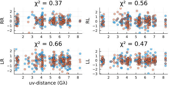
Now let's evaluate our fits by plotting the residuals

using Plots
residual(post, xopt)

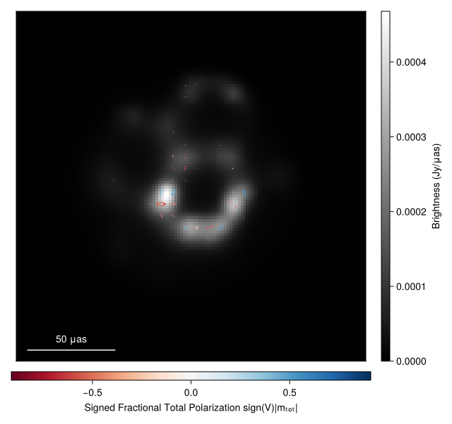
These look reasonable, although there may be some minor overfitting. Let's compare our results to the ground truth values we know in this example. First, we will load the polarized truth

imgtrue = load_fits(joinpath(__DIR, "..", "..", "Data", "polarized_gaussian.fits"), IntensityMap{StokesParams})

╭─────────────────────────────────────────────────╮
│ 1024×1024 IntensityMap{StokesParams{Float64},2} │
├─────────────────────────────────────────────────┴────────────────────── dims ┐
  ↓ X Sampled{Float64} LinRange{Float64}(-4.843402302490755e-10, 4.843402302490755e-10, 1024) ForwardOrdered Regular Points,
  → Y Sampled{Float64} LinRange{Float64}(-4.843402302490772e-10, 4.843402302490772e-10, 1024) ForwardOrdered Regular Points
├──────────────────────────────────────────────────────────────────── metadata ┤
  ComradeBase.MinimalHeader{Float64}("SgrA", 266.4168370833333, -28.99218944444445, 51544.0, 2.3e11)
└──────────────────────────────────────────────────────────────────────────────┘
  ↓ →          …  4.8434e-10
 -4.8434e-10       [6.86545e-65, 4.08459e-78, 1.02982e-65, 1.02982e-66]
 -4.83393e-10      [8.99558e-65, 5.35191e-78, 1.34934e-65, 1.34934e-66]
 -4.82446e-10      [1.17804e-64, 7.00873e-78, 1.76706e-65, 1.76706e-66]
  ⋮            ⋱  
  4.82446e-10      [1.17804e-64, 7.00873e-78, 1.76706e-65, 1.76706e-66]
  4.83393e-10      [8.99558e-65, 5.35191e-78, 1.34934e-65, 1.34934e-66]
  4.8434e-10       [6.86545e-65, 4.08459e-78, 1.02982e-65, 1.02982e-66]

Select a reasonable zoom in of the image.

imgtruesub = regrid(imgtrue, imagepixels(fovx, fovy, nx*4, ny*4))
img = intensitymap(Comrade.skymodel(post, xopt), axisdims(imgtruesub))

#Plotting the results gives
import CairoMakie as CM
fig = imageviz(img, adjust_length=true, colormap=:bone, pcolormap=:RdBu)
fig |> DisplayAs.PNG |> DisplayAs.Text

Note

The image looks a little noisy. This is an artifact of the MAP image. To get a publication quality image we recommend sampling from the posterior and averaging the samples. The results will be essentially identical to the results from EHTC VII.

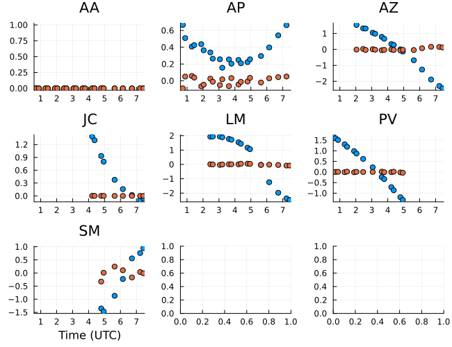
We can also analyze the instrument model. For example, we can look at the gain ratios and products. To grab the ratios and products we can use the caltable function which will return analyze the gprat array and convert it to a uniform table. We can then plot the gain phases and amplitudes.

gphase_ratio = caltable(xopt.instrument.gprat)
gamp_ratio   = caltable(exp.(xopt.instrument.lgrat))

───────────────────────────────────────────────────┬────────────────────────────
                                              time │       AA        AP        ⋯
───────────────────────────────────────────────────┼────────────────────────────
 IntegrationTime{Float64}(57854, 0.583333, 0.0002) │  1.00194   missing   miss ⋯
 IntegrationTime{Float64}(57854, 0.733333, 0.0002) │ 0.999826   1.00024   miss ⋯
 IntegrationTime{Float64}(57854, 0.883333, 0.0002) │ 0.997493  0.998955   miss ⋯
      IntegrationTime{Float64}(57854, 1.3, 0.0002) │  1.00175   1.00021   miss ⋯
     IntegrationTime{Float64}(57854, 1.45, 0.0002) │ 0.999504   1.00003   miss ⋯
  IntegrationTime{Float64}(57854, 1.89167, 0.0002) │  1.00283  0.997662   miss ⋯
  IntegrationTime{Float64}(57854, 2.04167, 0.0002) │ 0.998637   1.00067   1.00 ⋯
  IntegrationTime{Float64}(57854, 2.45833, 0.0002) │ 0.999901   1.00031  0.995 ⋯
   IntegrationTime{Float64}(57854, 2.6125, 0.0002) │   1.0009  0.999168   1.00 ⋯
  IntegrationTime{Float64}(57854, 3.05833, 0.0002) │  1.00369  0.999999  0.999 ⋯
  IntegrationTime{Float64}(57854, 3.20833, 0.0002) │ 0.996872    0.9995        ⋯
    IntegrationTime{Float64}(57854, 3.625, 0.0002) │ 0.997069   1.00267  0.998 ⋯
  IntegrationTime{Float64}(57854, 3.77917, 0.0002) │  1.00282  0.997491   1.00 ⋯
    IntegrationTime{Float64}(57854, 4.225, 0.0002) │ 0.997503  0.997454  0.998 ⋯
    IntegrationTime{Float64}(57854, 4.375, 0.0002) │  1.00298  0.999742    0.9 ⋯
  IntegrationTime{Float64}(57854, 4.79167, 0.0002) │  1.00308  0.995933   1.00 ⋯
                         ⋮                         │    ⋮         ⋮         ⋮  ⋱
───────────────────────────────────────────────────┴────────────────────────────
                                                    5 columns and 6 rows omitted

Plotting the phases first, we see large trends in the righ circular polarization phase. This is expected due to a lack of image centroid and the absense of absolute phase information in VLBI. However, the gain phase difference between the left and right circular polarization is stable and close to zero. This is expected since gain ratios are typically stable over the course of an observation and the constant offset was removed in the EHT calibration process.

gphaseR = caltable(xopt.instrument.gpR)
p = Plots.plot(gphaseR, layout=(3,3), size=(650,500));
Plots.plot!(p, gphase_ratio, layout=(3,3), size=(650,500));
p |> DisplayAs.PNG |> DisplayAs.Text

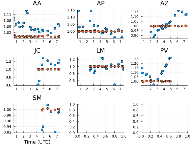
Moving to the amplitudes we see largely stable gain amplitudes on the right circular polarization except for LMT which is known and due to pointing issues during the 2017 observation. Again the gain ratios are stable and close to unity. Typically we expect that apriori calibration should make the gain ratios close to unity.

gampr = caltable(exp.(xopt.instrument.lgR))
p = Plots.plot(gampr, layout=(3,3), size=(650,500))
Plots.plot!(p, gamp_ratio, layout=(3,3), size=(650,500))
p |> DisplayAs.PNG |> DisplayAs.Text

To sample from the posterior, you can then just use the sample function from AdvancedHMC like in the other imaging examples. For example

using AdvancedHMC
chain = sample(rng, post, NUTS(0.8), 10_000, n_adapts=5000, progress=true, initial_params=xopt)

---

This page was generated using Literate.jl.

---

1. Hamaker J.P, Bregman J.D., Sault R.J. (1996) [https://articles.adsabs.harvard.edu/pdf/1996A%26AS..117..137H] ↩︎

2. Pesce D. (2021) [https://ui.adsabs.harvard.edu/abs/2021AJ....161..178P/abstract] ↩︎